Download
1 / 70
730 likes | 1.01k Views
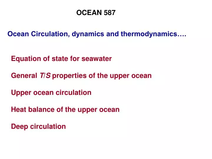
OCEAN 587. Ocean Circulation, dynamics and thermodynamics…. Equation of state for seawater General T / S properties of the upper ocean Upper ocean circulation Heat balance of the upper ocean Deep circulation. = ( S , T , p , ……). [Determined from laboratory experiments].

E N D
OCEAN 587 Ocean Circulation, dynamics and thermodynamics…. Equation of state for seawater General T/S properties of the upper ocean Upper ocean circulation Heat balance of the upper ocean Deep circulation
= (S, T, p, ……) [Determined from laboratory experiments] [ S = salinity; T = temperature; p = pressure ] In order to use this relation to infer it is necessary to clearly define the meanings of S, T, and p.
Salinity…. Why is the ocean salty? [ A great question ] Hydrological cycle fresh water precipitation continental runoff evaporation salinity [seems unlikely] Geochemical implications: Earth’s crust is rich in aluminum; rivers are rich in carbonates; oceans are rich in halides and sulfides. Seawater is a complex chemical system that contains traces of nearly all naturally occurring elements. The dissolved part of seawater is about 78% NaCl by mass.
The chemical composition of seawater…. Amazingly, the proportions of the major constituents of seawater are nearly constant everywhere.
This constancy of proportions means that to a good approximation, only one component of seawater needs to be measured, and all of the other can be inferred from it. (what are the limitations?) Instead of characterizing a seawater sample by knowing all of its chemical components, we can characterize the sample by a single parameter. We shall call this parameter the salinity. Formal, traditional definition of salinity: “The total amount of solid materials in grams contained in one kilogram of seawater when all the carbonate has been converted to oxide, the bromine and iodine replaced by chlorine, and all organic matter completely oxidized.”
34.60 34.70 34.72 How well do we need to measure S? The section of S along 43 S in the S. Pacific shows that there is considerable detail at signal levels 0.01 PSU.
Temperature (continued)…. Seawater is slightly compressible. What are the implications of this? [warming] [cooling] Adiabatic changes in temperature: changes in temperature when there are no changes in heat.
Temperature (continued)…. Potential temperature (): the temperature that a seawater parcel would have if it were raised adiabatically to the sea surface. [Note: T ] The temperature change in adiabatic conditions is due to compressibility alone, since seawater is slightly compressible…..this can get confusing. Given 2 parcels, which is heavier? Care must be taken, since they are at different pressures. Solution: refer both to a common pressure.
Temperature (continued)…. T In situ temperature T increases as depth inceases. Potential temperature does not increase with depth.
Density…. = (S, T, p) is the symbolic equation of state. Over the water column, varies by a few per cent. surf 1.021 g/cm3 ; bot 1.071 g/cm3 [typical values] In the upper ocean, (S, T) . In the deep sea, (p) . Define the parameter as a more useful representation of density: = ( 1) 1000 (cgs) ; = 1000 (mks)
There are several different types of density…. • = (S, T, p) (in situ sigma) • t = (S, T, 0) (“sigma-tee”) • = (S, , 0) (“sigma-theta”) • note: • (4) po = (S, po, po) [po = (S, T, po) ] [potential temperature] [ = adiabatic lapse rate = T/p ]
Typical profiles in the ocean…. [ from Ocean Station P, 50N, 145W ] t T S
Equation of state…. Step 1, fresh water equation Step 2, add salinity at zero pressure Step 3, full equation with T, S, p [a 29 term polynomial]
Equation of state…. The equation of state for seawater is nonlinear. This has major implications to ocean mixing.
Ocean circulation: surface currents…. [notice E/W asymmetry] [ 0-500 dbar dynamic ht; maximum range ~ 2 m]
The Heat Balance of the Earth (and the ocean’s role)…. Solar heating is ultimately the source of all energy at the Earth’s surface, except for tides and geothermal heating. The atmosphere and ocean exchange heat and energy in a complicated set of feedbacks. Recall the 2nd law of thermodynamics…. Heat is conserved.
Simple heat transfer…. 2 adjacent blocks Assume T1 > T2 Let Tf be the final temperature Heat lost from block 1 = m1c1(T1Tf) = H1 Heat gained by block 2 = m2c2(Tf T2) = H2 H1 = H2 Tf = (m1c1T1 + m2c2T2)/(m1c1 + m2c2)
Atmosphere-ocean heat transfer…. Suppose we change T in the lower 10 km of the atmosphere by 10 C (a massive change!). Suppose we put all of this heat into the upper 100 m of the ocean. How much would T in the upper 100 m of the ocean change? Atmosphere Ocean (.0013) (10) (0.25) (10) (1) (0.1) (1) (?) [small! the ocean acts as a buffer to the atmosphere] result:
The heat content in the upper 300 m of the ocean has varied over the past 50 years, generally increasing…where has this heat come from? [heating rate 0.6 C/century] [from Levitus]
The concept of a flux…. area A amount ofstuff S per unit time The flux of S is defined as the amount of S crossing the area A per unit time; a flux is just (amount)/(area time).
The global heat balance (schematic)…. atmosphere ocean/land/cryosphere/biosphere
The heat balance of the ocean…. QT = QS + QB + QH + QE + QV + QG where QT = net heat input to the Earth ( 0 watts/m2) QS = direct solar input ( +150 watts/m2) QB = black body radiation (50 watts/m2) QH = sensible heat loss (10 watts/m2) QE = evaporative heat loss (90 watts/m2) QV = advective heat transport (0 watts/m2) QG = geothermal heating ( +0.01 watts/m2) [note: there are errors and uncertainties associated with each of these estimates]
QB, black body radiation…. [Sun 0.7 m] [Earth 15 m] Wien’s Law: maxT = A (a constant) Sun: high T (short ); Earth: low T (long )
QB, black body radiation…. The amount of heat radiated by a black-body of temperature T can be estimated from the Stefan-Boltzmann relation as QB = T4 , where is the Stefan-Boltzmann constant. For the case where there is no atmosphere and the heat balance is in equilibrium, on the Earth we would have QB = So (1-)/4 = T4T = (222/)1/4 278 K . This is too cold for the globally averaged T (actually about 300 K). [ = 5.67 10-8 W/(m2 K4) ]
The concept of flux-gradient diffusion…. [note: this is generally true in the molecular case only] The flux is proportional to the gradient of the concentration, with the constant of proportionality being the diffusivity .
QH, conductive (or sensible) heat flux…. Since the ocean is generally at a different temperature than the atmosphere, there will be a conduction of heat between them (recall the two blocks). Fourier’s Law of heat conduction: F T or F = K T [K = diffusivity] So, QH = c T/z, c = CpK [this is an empirical result]
QH, continued…. Note 1: K = K (T, wind, sea state, humidity…..) 10 – 103 cm2/sec at the sea surface Note 2: Strictly, the concept of a diffusivity K only applies to laminar flows. Where turbulence occurs (everywhere !), this formulation serves as a parameterization only (“eddy diffusivity”).
QH for the Pacific…. [note the east-west asymmetry]
Evaporative heat flux, QE…. The latent heat of evaporation L for fresh water is L = 2494 joules/kg @ 2 C This much energy must be supplied in order for the state transition from liquid to vapor to occur. In the oceanic case, the energy will be extracted from surface seawater in the form of heat, thus having a net cooling effect. This evaporated seawater will appear as water vapor in the atmosphere, and the latent heat L will be released into the atmosphere upon condensation of the water vapor.
QE, continued…. Note: QE is generally the largest term in the heat balance equation, after direct solar input QS. How can QE be estimated? In general the evaporation rate and associated heat flux are a complicated function of a number of variables and can only be estimated empirically, QE = QE(Toc, Tatm, S, wind, sea state, humidity,….) Many estimates of the evaporative heat flux exist, using a variety of parameterizations. Estimated errors are not small, in general.
QE for the Pacific…. [note the east-west asymmetry]
The heat balance…. QT = QS + QB + QH + QE + QV + QG = 0 = Qsurf + QV + QG Qsurf + QV = 0 where Qsurf = QS + QB + QH + QE What is the total surface heat flux from the ocean, Qsurf ?
Qsurf for the Pacific…. [note east-west asymmetry]
Global heating at the sea surface…. QS QE QH
Qsurffor the Atlantic…. [note east-west asymmetry] (watts/m2) -150 -250 0 -75 -50 -100
QV , advective heat flux…. Qsurf + QV= 0 [Globally, QV = 0, but this might not be true locally.] If there is a gain or loss of heat from the sea surface, then the ocean must export or import heat in order to keep the system in thermodynamical equilibrium. Result: Ocean Circulation. [The integration proceeds over the surface area of a sector of ocean, including the surface, sidewalls, and the bottom.] Thus,
QV, continued…. an ocean losing/gaining heat at the sea surface an ocean losing/gaining heat via advection through the sides
QV, continued…. + flux in, flux out (1) (2) If (1) > 0 (ocean gains heat from the atmosphere), then (2) < 0 (ocean circulation must transport heat away) If (1) < 0 (ocean loses heat to the atmosphere), then (2) > 0 (ocean circulation must transport heat in) Globally, the surface heat budget for the ocean has been estimated from bulk formulae, marine observations, satellites, etc. If we have an estimate of Qsurf, we should be able to estimate Qv.
QV continued…. units: 1013 watts Global ocean heat transport, basin integrated
QV, averaged along latitude by ocean…. [note: Atlantic is different]
QV(continued)…. Parameterization of Qv : Let V equal a velocity normal to some surface, and let T be the temperature of the water flowing with V. The heat transport associated with V and T is then QV = CVT where C is the heat capacity and the density. Check the units: [heat/area/time, a flux by definition]
QV , continued…. [note: T is measured relative to some reference temperature] QV = CVT Note the meaning of this parameterization: Increasing either the temperature, or the flow, will increase the heat transport. Also note that warm water flowing north = cold water flowing south (T>0, V>0) (T<0, V<0) [consider the Atlantic]
QV , continued…. Ocean Atmosphere Total Northward heat transport by the ocean and atmosphere
QV, continued…. Hydrographic lines in the World Ocean Circulation Experiment (WOCE)
Ocean circulation: surface currents…. [notice E/W asymmetry] [ 0-500 dbar dynamic ht; maximum range ~ 2 m]