Download
1 / 11
310 likes | 2.18k Views
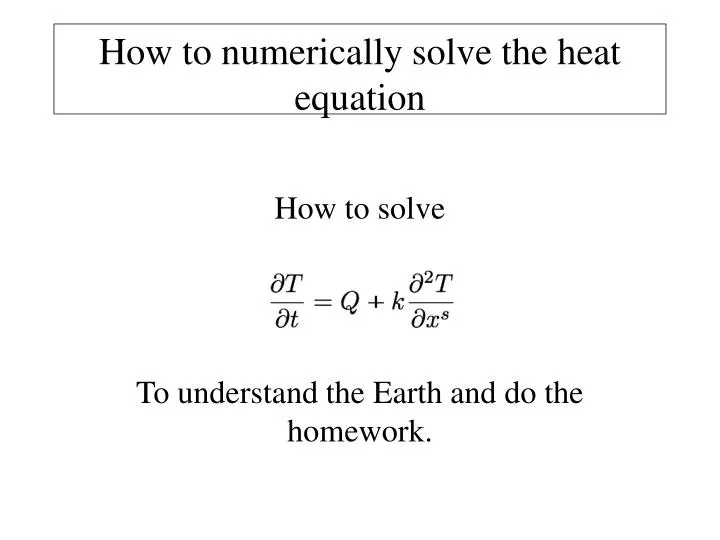
How to numerically solve the heat equation. How to solve To understand the Earth and do the homework. How do we think about the continous problem? think about "heat flux;" proportional to so so what is dT/dt? difference between at either end this is if k is constant, so:.

E N D
How to numerically solve the heat equation How to solve To understand the Earth and do the homework.
How do we think about the continous problem? • think about "heat flux;" proportional to • so • so what is dT/dt? • difference between at either end • this is • if k is constant, so:
Why is it an ODE again? • Now we can solve it with Runge-Kutta • In the homework, you must implement the above equation, without Q, in heat_eq.m • You will want to use the "end" notation, so that (Ti-Ti-1) • Becomes T(2:end)-T(1:end-1) • But if T is 200 rows by 1 column, what is T(2:end)-T(1:end-1)? • What to do about this? See next slide!
Remember the boundary conditions! • T=something at boundary • or insulating boundary • Pad the T vector with the boundary conditions! Tpad=[Tbc1 ; T ; TbcN] • What will Tbc be if the boundary is insulating? • What if you want to set the boundary to a temperature? • If you do this correctly, the length of the vectors will come out correctly! demonstrate with
Other things to learn: In ode23 and ode45, we must give it a function that takes as an argument time and a vector • you can see this on the next page • How can you share other data with it? • for example the spacing z and the depth of the soil?
Explain "global" variables % heat_driver.m % this is a driver for the a simple ode_based heat equation discussed % in class. There is NO radioactive heating in this solver. clear all clf() % Define the grid spacing, dz, and the domain over which we % calculate the soil temperature. Both in units of length. % % Make these global, so we can access them in heat_eq.m global dz zvec dz=0.05; %units of meters zvec=-[0:dz:20]'; %must be a column vector. …. %run simulation; [t_sol,T_sol]=ode23(@heat_eq,t_span,T0); function dTdt=heat_eq(t,T); % this code solves the heat equation over the domain defined by the % grid-spacing dz and the vector of distance zvec; both of these are % global variables, and must be defined outside of this routine. % % the boundary conditions for the code are defined below, % The grid must be defined elsewhere; dz is the grid spacing, and zvec % is a vector defining the z-coordinate. % global dz zvec
contour() makes plots with just lines, • contourf() fills in colors • and colorbar() makes a color bar contour(x_axis_vec,y_axis_vec,data,vector_contour_intervals) • Thus subplot(2,1,1) contourf(t_sol/(365.25*8.64e4),zvec,T_sol',[-4.8:0.25:21.5]); shading flat %explain colorbar() %explain xlabel('Time, in years') ylabel('Distance') • Why the transpose on T_sol?
Now lets do the homework! • Next time, more discussion of what the heat equation / diffusion equation tells us about the world.