Download
1 / 26
280 likes | 678 Views
Stochastic Loss Reserving with the Collective Risk Model. Glenn Meyers ISO Innovative Analytics Casualty Loss Reserving Seminar September 18, 2008. Outline of Presentation. General Approach to Stochastic Modeling Allows for better estimate of the mean Quantify uncertainty in estimate

E N D
Stochastic Loss Reserving with the Collective Risk Model Glenn Meyers ISO Innovative Analytics Casualty Loss Reserving Seminar September 18, 2008
Outline of Presentation • General Approach to Stochastic Modeling • Allows for better estimate of the mean • Quantify uncertainty in estimate • The Paper - “Stochastic Loss Reserving with the Collective Risk Model”
Introduce Stochastic Modeling with an Example • X ~ lognormal with m = 5 and s = 2 • Two ways to estimate E[X] (= 1,097) • Straight Average – • Lognormal Average – where
Which Estimator is Better? EN[X] or EL[X]? • Straight Average, EN[X], is simple. • Lognormal Average, EL[X] is complicated. • But derived from the maximum likelihood estimator for the lognormal distribution • Evaluate by a simulation • Sample size of 500 • 2,000 samples • Look at the variability of each estimator
Results of Simulation • Confidence interval is narrower • No outrageous outliers
Lesson from Example • Knowing the distribution of the observations can lead to a better estimate of the mean! • Actuaries have long recognized this. • Longtime users of robust statistics • Calculate basic limit average severity • Fit distributions to get excess severity • More recently recognized in the growing use of the Generalized Linear Model
Parameter Uncertaintyand the Gibbs Sampler • Gibbs sampler is often used for Bayesian analyses. • It randomly generates parameters in proportion to posterior probabilities. • Parameters randomly fed into the sampler in proportion to prior probabilities. • Accepted in proportion to • Results in the posterior distribution of parameters.
Gibbs Sampler on a LognormalExample from February 2008 Actuarial Review • Simulate m and s from a prior distribution of parameters. • Calculate the likelihood of each simulated m and s. • Select a random uniform number U. • Accept m and s into the posterior distribution if
Posterior Distribution of m and s is Only of Temporary Interest! • Most often we are interested in functions of m and s. • For example: Mean Limited Expected Value
Some posterior parameters generated by Gibbs sampler Layer Expected Value25,000 to 30,000
Evolving Strategy for Modeling Uncertainty • Point Estimates • Based on MLE or (Bayesian) Predictive Mean • Ranges - Bayesian • “Quantities of Interest” weighted by posterior probabilities of the parameters • Discrete prior or Gibbs Sampler • Some Applications • Claim severity models – COTOR Challenge • Loss reserve models – Today’s topic
S&P Report, November 2003Insurance Actuaries – A Crisis in Credibility “Actuaries are signing off on reserves that turn out to be wildly inaccurate.”
Prior Work on Loss Reserve Models • Estimating Predictive Distributions for Loss Reserve Models – 2006 CLRS and Variance • Initial application of the strategy to loss reserves • Tested results on subsequent loss payments • Set a standard for evaluating loss reserve formulas • Thinking Outside the Triangle – 2007 ASTIN Colloquium • Tested a formula based on simulated outcomes • Provided an example • Model parameters from MLE understated range • Bayesian mixing (spreading out) provided accurate range
Stochastic Loss Reserving with the Collective Risk Model • Focuses mainly on “How to do it” • “Data” is simulated from collective risk model • Code for implementing algorithms included • Secondary Objective • Use Gibbs sampler (as does Verrall in Variance)
Method Illustrated on Data Incremental Paid Losses
Plan of Attack • Specify stochastic model needed to calculate likelihood of the data • Calculate MLE and parameters for Gibbs sample • Quantity of Interest = Percentiles of OS Loss
Model for Expected Losses • Two models for expected loss • Cape Cod Model • Beta Model • {ELRAY} and {DevLag} and/or {a,b} parameters estimated from data
Need a Stochastic Model to Calculate Likelihoods Use the collective risk model. • Select a random claim count, NAY,Lag from a Poisson distribution with mean l. • For i = 1, 2, …, NAY,Lag, select a random claim amount, ZLag,i. • Set, or if NAY,Lag = 0, then XAY,Lag = 0..
Details of Distributions • Pareto severity distribution • for all lags – a = 2 • Table of q’s • Severity increases with lag • Approximate likelihood calculated by matching moments with an overdispersed negative binomial distribution (for now).
Bayesian AnalysesSpecify Prior Distributions • Prior parameters were derived from looking at “Estimating Predictive Distributions … “ paper. Beta Model Cape Cod Model
Graphical Representation of Gibbs Sample – Cape Cod Model Note that the posteriors are tighter, showing how the data narrows the range of results.
Graphical Representation of Gibbs Sample – Beta Model Note that the coefficient of variation decreases as we get more paid data.
Quantity of InterestPredictive Distributions of Reserve Outcomes • Collective risk model • Simulation • Randomly select {ELRi} and {Devj} • Simulate as done above. • Use a Fast Fourier Transform • Faster, more accurate, but uses some math • Used in the paper
Quantity of InterestPredictive Distributions of Reserve Outcomes Cape Cod Model Mean = 60,871 StDev = 5,487 Beta Model Mean = 67,183 StDev = 5,605