Download

1 / 37
370 likes | 408 Views
Backpropagation. Multilayer Perceptron. Function Approximation. The following example will illustrate the flexibility of the multilayer perceptron for implementing functions. The network output response for these parameters as the input P is varied over the range [-2, 2].

E N D
Function Approximation The following example will illustrate the flexibility of the multilayer perceptron for implementing functions.
The network output response for these parameters as the input P is varied over the range [-2, 2].
Notice that the response consists of two steps, one for each of the log-sigmoid neurons in the first layer. By adjusting the network parameterswe can change the shape and location of each step.The centers of the steps occur where the net input to a neuron in the first layer is zero: Step n1=0 Step n2=0 The steepness of each step can be adjusted by changing the network weights.
The blue curve is the nominal response. The other curves correspond to the network response when one parameterat a time is varied over the following ranges
Effect of Parameter Changes on Network Response The biases in the first (hidden) layer can be used to locate the position of the steps. • In fact, any two-layer networks, with sigmoid transfer functions in the hidden layer and linear transfer functions in the output layer, can approximate virtually any function of interest to any degree of accuracy, provided sufficiently many hidden units are available. • The next step is to develop an algorithm to train such networks. The weights determine the slope of the steps. The bias in the second (output) layer shifts the entire network response up or down.
The Backpropagation Algorithm Multilayer network The neurons in the first layer receive external inputs: M is the number of layers in the net The outputs of the neurons in the last layer are considered the net outputs
Performance Index of Backpropagation • The performance index of the algorithms is the mean square error. (Least Mean Square error or LMS). • The weights are adjusted, using a gradient descent method, so as to minimize the mean square error. • The algorithm is provided with a set of examples of proper network behavior: • where pq is an input to the network, and tq is the corresponding target output. • As each input is applied to the network, the network output is compared to the target.
The algorithm should adjust the network parameters in order to minimize the mean square error: • where E[ ] denotes the expected value, and x is the vector of network weights and biases • If the network has multiple outputs this generalizes to the vector case • Approximate Mean Square Error (the expectation replaced by single iteration k) Where is the estimated performance index.
Now we come to the difficult part – the computation of the partial derivatives. • For a single-layer linear network these partial derivatives are conveniently computed. • For the multilayer network the error is not an explicit function of the weights in the hidden layers, therefore these derivatives are not computed so easily. • Because the error is an indirect function of the weights in the hidden layers, we will use the chain rule of calculus to calculate the derivatives. • To review the chain rule, suppose that we have a function f that is an explicit function only of the variablen. • We want to take the derivative of f with respect to a third variablew. The chain rule is then:
Gradient Calculation • The second term in each of these equations can be easily computed, since the net input to layer is an explicit function of the weights and bias in that layer: ˆ Sensitivitysim: the sensitivity of F to changes in the ith element of the net input n at layer m
Steepest Descent • We can now express the approximate steepest descent algorithm as
Backpropagating the Sensitivities • It now remains for us to compute the sensitivities sm, which requires another application of the chain rule. • It is this process that gives us the term backpropagation, because it describes a recurrence relationship in which the sensitivity at layer m is computed from the sensitivity at layer m+1. • To derive the recurrence relationship for the sensitivities, we will use the following Jacobian matrix:
Example: Function Approximation • To illustrate the backpropagation algorithm, let’s choose a 1-2-1 network to approximate the function
Initial Conditions • Before we begin the backpropagation algorithm we need to choose some initial values for the network weights and biases. Generally these are chosen to be small random values. • To obtain our training set we will evaluate this function at several values of p. • Next, we need to select a training set: {p1, t1}, {p2, t2, …, {pq, tq} . • In this case, we will sample the function at 21 points in the range [-2,2] at equally spaced intervals of 0.2. .
Network Response • The response of the network for these initial values is as shown, along with the sine function we wish to approximate. • The training points are indicated by the circles
Forward Propagation • The training points can be presented in any order, but they are often chosen randomly. • For our initial input we will choose p=1, which is the 16th training point: a0 = p = 1 • The output of the first layer is then
The error would then be • The second layer output is
Transfer Function Derivatives • The next stage of the algorithm is to backpropagate the sensitivities. • Before we begin the backpropagation, we will need the derivatives of the transfer functions f1(n), and f2(n) • For the first layer • For the second layer we have
Backpropagation • We can now perform the backpropagation. The starting point is found at the second layer:
How to complete the training • Up to this the first iteration of the back propagation algorithm is completed. • We next proceed to randomly choose another input from the training set and perform another iteration of the algorithm. • We continue to iterate until the difference between the network response and the target function reaches some acceptable level. • (Note that this will generally take many passes through the entire training set.)
Batch vs. Incremental Training • The algorithm described above is the stochastic gradient descent algorithm, which involves “on-line” or incremental training, in which the network weights and biases are updated after each input is presented . • It is also possible to perform batch training, in which the complete gradient is computed (after all inputs are applied to the network) before the weights and biases are updated. • For example, if each input occurs with equal probability, the mean square error performance index can be written
Therefore, to implement a batch version of the backpropagation algorithm, we would step from the forward Eqs. through the sensitive calculations for all of the inputs in the training set. • Then, the individual gradients would be averaged to get the total gradient. • The update equations for the batch steepest descent algorithm would then be
Choice of Network Architecture • For our first example let’s assume that we want to approximate the following functions: • where i takes on the values 1, 2, 4 and 8. • As i is increased, the function becomes more complex, because we will have more periods of the sine wave over the interval -2 ≤ p ≤ 2. • It will be more difficult for a neural network with a fixed number of neurons in the hidden layers to approximate g(p) as i is increased. • For this first example we will use a 1-3-1 network, • The transfer function for the first layer is log-sigmoid and the transfer function for the second layer is linear. • This type of two-layer network can produce a response that is a sum of three log-sigmoid functions (or as many log-sigmoids as there are neurons in the hidden layer). • Clearly there is a limit to how complex a function this network can implement.
The final network responses after it has been trained are shown by the blue lines
We can see that for i=4 the 1-3-1 network reaches its maximum capability. • When i>4 the network is not capable of producing an accurate approximation
Choice of Network Architecture (1-S1-1), the response of this network is a superposition of S1 sigmoid functions
To summarize these results: • a 1- S1 -1 network, with sigmoid neurons in the hidden layer and linear neurons in the output layer, can produce a response that is a superposition of S1 sigmoid functions. • If we want to approximate a function that has a large number of inflection points, we will need to have a large number of neurons in the hidden layer.