Hinrich Schütze and Christina Lioma Lecture 5: Index Compression

1. HinrichSchütze and Christina Lioma Lecture 5: Index Compression

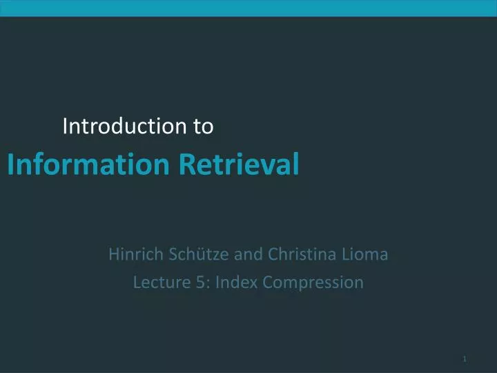
2. Overview • Recap • Compression • Term statistics • Dictionary compression • Postings compression

3. Outline • Recap • Compression • Term statistics • Dictionary compression • Postings compression

4. BlockedSort-BasedIndexing 4

5. Single-pass in-memoryindexing • Abbreviation: SPIMI • Key idea 1: Generate separate dictionaries for each block – no need to maintain term-termID mapping across blocks. • Key idea 2: Don’t sort. Accumulate postings in postings lists astheyoccur. • With these two ideas we can generate a complete inverted indexforeach block. • These separate indexes can then be merged into one big index. 5

6. SPIMI-Invert 6

7. MapReduceforindexconstruction 7

8. Dynamic indexing: Simplestapproach • Maintain big main index on disk • New docs go into small auxiliary index in memory. • Search across both, merge results • Periodically, merge auxiliary index into big index 8

9. Roadmap • Today: indexcompression • Next 2 weeks: perspective of the user: how can we give the user relevant results, how can we measure relevance, what types of user interactions are effective? • After Pentecost: statistical classification and clustering in informationretrieval • Last 3 weeks: web information retrieval 9

10. Take-awaytoday • Motivation forcompression in informationretrievalsystems • How can we compress the dictionary component of the invertedindex? • How can we compress the postings component of the inverted index? • Term statistics: how are terms distributed in document collections? 10

11. Outline • Recap • Compression • Term statistics • Dictionary compression • Postings compression

12. Whycompression? (in general) • Use less disk space (saves money) • Keep more stuff in memory (increases speed) • Increase speed of transferring data from disk to memory (again, increasesspeed) • [read compressed data and decompress in memory] isfasterthan [readuncompresseddata] • Premise: Decompressionalgorithmsare fast. • This is true of the decompression algorithms we will use. 12

13. Whycompression in informationretrieval? • First, we will consider space for dictionary • Main motivation for dictionary compression: make it small enough to keep in main memory • Then for the postings file • Motivation: reduce disk space needed, decrease time needed to readfromdisk • Note: Large search engines keep significant part of postings in memory • We will devise various compression schemes for dictionary and postings. 13

14. Lossy vs. losslesscompression • Lossy compression: Discard some information • Several of the preprocessing steps we frequently use can be viewedaslossycompression: • downcasing, stop words, porter, number elimination • Lossless compression: All information is preserved. • What we mostly do in index compression 14

15. Outline • Recap • Compression • Term statistics • Dictionary compression • Postings compression

16. Model collection: The Reuters collection 16

17. Effect of preprocessing for Reuters 17

18. How big is the term vocabulary? • That is, how many distinct words are there? • Can we assume there is an upper bound? • Not really: At least 7020 ≈ 1037 different words of length 20. • The vocabulary will keep growing with collection size. • Heaps’ law: M = kTb • M is the size of the vocabulary, T is the number of tokens in thecollection. • Typical values for the parameters k and b are: 30 ≤ k ≤ 100 andb ≈ 0.5. • Heaps’ law is linear in log-log space. • It is the simplest possible relationship between collection size and vocabulary size in log-log space. • Empiricallaw 18

19. Heaps’ lawfor Reuters Vocabulary size M as a functionofcollectionsize T (number of tokens) for Reuters-RCV1. Forthese data, thedashedline log10M = 0.49 ∗ log10T + 1.64 is the best least squares fit. Thus, M = 101.64T0.49 and k = 101.64 ≈ 44 and b = 0.49. 19

20. Empirical fit for Reuters • Good, as we just saw in the graph. • Example: for the first 1,000,020 tokens Heaps’ law predicts 38,323 terms: • 44 × 1,000,0200.49 ≈ 38,323 • The actual number is 38,365 terms, very close to the prediction. • Empirical observation: fit is good in general. 20

21. Exercise • What is the effect of including spelling errors vs. automatically correcting spelling errors on Heaps’ law? • Compute vocabulary size M • Looking at a collection of web pages, you find that there are 3000 different terms in the first 10,000 tokens and 30,000 different terms in the first 1,000,000 tokens. • Assume a search engine indexes a total of 20,000,000,000 (2 × 1010) pages, containing 200 tokens on average • What is the size of the vocabulary of the indexed collection as predictedby Heaps’ law? 21

22. Zipf’slaw • Now we have characterized the growth of the vocabulary in collections. • We also want to know how many frequent vs. infrequent terms we should expect in a collection. • In natural language, there are a few very frequent terms and very many very rare terms. • Zipf’s law: The ith most frequent term has frequency cfiproportional to 1/i . • cfi is collection frequency: the number of occurrences of the term tiin the collection. 22

23. Zipf’slaw • Zipf’s law: The ith most frequent term has frequency proportional to 1/i . • cf is collection frequency: the number of occurrences of the term in thecollection. • So if the most frequent term (the) occurs cf1 times, then the second most frequent term (of) has half as many occurrences • . . . and the third most frequent term (and) has a third as manyoccurrences • Equivalent: cfi= cikand log cfi= log c +k log i (fork = −1) • Example of a power law 23

24. Zipf’slawfor Reuters Fit is not great. What isimportantisthe keyinsight: Fewfrequent terms, many rare terms. 24

25. Outline • Recap • Compression • Term statistics • Dictionary compression • Postings compression

26. Dictionarycompression • The dictionary is small compared to the postings file. • But we want to keep it in memory. • Also: competition with other applications, cell phones, onboard computers, fast startup time • So compressing the dictionary is important. 26

27. Recall: Dictionary as array of fixed-width entries • Space needed: 20 bytes 4 bytes 4 bytes • for Reuters: (20+4+4)*400,000 = 11.2 MB 27

28. Fixed-widthentriesarebad. • Most of the bytes in the term column are wasted. • We allot 20 bytes for terms of length 1. • Wecan’t handle HYDROCHLOROFLUOROCARBONS and SUPERCALIFRAGILISTICEXPIALIDOCIOUS • Average length of a term in English: 8 characters • How can we use on average 8 characters per term? 28

29. Dictionaryas a string 29

30. Space for dictionary as a string • 4 bytes per term for frequency • 4 bytes per term for pointer to postings list • 8 bytes (on average) for term in string • 3 bytes per pointer into string (need log2 8 · 400000 < 24 bits to resolve 8 · 400,000 positions) • Space: 400,000 × (4 +4 +3 + 8) = 7.6MB (compared to 11.2 MB forfixed-widtharray) 30

31. Dictionary as a string with blocking 31

32. Space for dictionary as a string with blocking • Example block size k = 4 • Where we used 4 × 3 bytes for term pointers without blocking . . . • . . .we now use 3 bytes for one pointer plus 4 bytes for indicating the length of each term. • We save 12 − (3 + 4) = 5 bytes per block. • Total savings: 400,000/4 ∗ 5 = 0.5 MB • This reduces the size of the dictionary from 7.6 MB to 7.1 • MB. 32

33. Lookup of a term without blocking 33

34. Lookup of a term with blocking: (slightly) slower 34

35. Front coding One block in blocked compression (k = 4) . . . 8 a u t o m a t a 8 a u t o m a t e 9 a u t o m a t i c 10 a u t o m a t i o n ⇓ . . . further compressed with front coding. 8 a u t o m a t ∗ a 1 ⋄ e 2 ⋄ i c 3 ⋄ i o n 35

36. Dictionary compression for Reuters: Summary 36

37. Exercise • Which prefixes should be used for front coding? What are the tradeoffs? • Input: list of terms (= the term vocabulary) • Output: list of prefixes that will be used in front coding 37

38. Outline • Recap • Compression • Term statistics • Dictionary compression • Postings compression

39. Postingscompression • The postings file is much larger than the dictionary, factor of at least 10. • Key desideratum: store each posting compactly • A posting for our purposes is a docID. • For Reuters (800,000 documents), we would use 32 bits per docID when using 4-byte integers. • Alternatively, we can use log2 800,000 ≈ 19.6 < 20 bits per docID. • Our goal: use a lot less than 20 bits per docID. 39

40. Key idea: Store gaps instead of docIDs • Each postings list is ordered in increasing order of docID. • Examplepostingslist: COMPUTER: 283154, 283159, 283202, . . . • It suffices to store gaps: 283159-283154=5, 283202-283154=43 • Example postings list using gaps : COMPUTER: 283154, 5, 43, . . . • Gaps for frequent terms are small. • Thus: We can encode small gaps with fewer than 20 bits. 40

41. Gap encoding 41

42. Variable lengthencoding • Aim: • For ARACHNOCENTRIC and other rare terms, we will use about 20 bits per gap (= posting). • For THE and other very frequent terms, we will use only a few bits per gap (= posting). • In order to implement this, we need to devise some form of variable lengthencoding. • Variable length encoding uses few bits for small gaps and many bits for large gaps. 42

43. Variable byte (VB) code • Used by many commercial/research systems • Good low-tech blend of variable-length coding and sensitivity to alignment matches (bit-level codes, see later). • Dedicate 1 bit (high bit) to be a continuation bit c. • If the gap G fits within 7 bits, binary-encode it in the 7 available bits and set c = 1. • Else: encode lower-order 7 bits and then use one or more additional bytes to encode the higher order bits using the same algorithm. • At the end set the continuation bit of the last byte to 1 (c = 1) and of the other bytes to 0 (c = 0). 43

44. VB codeexamples 44

45. VB codeencodingalgorithm 45

46. VB codedecodingalgorithm 46

47. Other variable codes • Instead of bytes, we can also use a different “unit of alignment”: 32 bits (words), 16 bits, 4 bits (nibbles) etc • Variable byte alignment wastes space if you have many small gaps – nibbles do better on those. • Recent work on word-aligned codes that efficiently “pack” a variable number of gaps into one word – see resources at the end 47

48. Gamma codes for gap encoding • You can get even more compression with another type of variable lengthencoding:bitlevelcode. • Gamma code is the best known of these. • First, we need unary code to be able to introduce gamma code. • Unarycode • Represent n as n 1s with a final 0. • Unary code for 3 is 1110 • Unary code for 40 is 11111111111111111111111111111111111111110 • Unary code for 70 is: • 11111111111111111111111111111111111111111111111111111111111111111111110 48

49. Gamma code • Represent a gap G as a pair of length and offset. • Offset is the gap in binary, with the leading bit chopped off. • For example 13 → 1101 → 101 = offset • Length is the length of offset. • For 13 (offset 101), this is 3. • Encode length in unary code: 1110. • Gamma code of 13 is the concatenation of length and offset: 1110101. 49

50. Gamma codeexamples 50