Download
1 / 44
440 likes | 506 Views
Learn about representational problems in computing due to limited precision bits and how to mitigate errors with parameterized types and functions. Explore complex numbers, characters, and operator overloading in Fortran 90.

E N D
Standard type sizes • Most machines store integers and reals in 4 bytes (32 bits) • Integers run from -2,147,483,648 to 2,147,483,647 • This is 232 • Single precision reals run from -1038 to 1038
Representational problem • Arithmetic errors are possible whenever real numbers are used in computing. • This is because only a limited number of bits are available to represent the exponent and mantissa of a real number. • The results are called • overflow errors, and • underflow errors
Roundoff error • roundoff error occurs whenever a real number must be approximated to fit into the alloted space. • For example: (A+B)2 - 2AB - B2 A2 A2 + 2AB + B2 - 2AB + B2 = A2 A2 = A2
Roundoff error • The result should be 1, but may not turn out that way due to rounding errors. (A+B)2 - 2AB - B2 A2 A2 + 2AB + B2 - 2AB + B2 = A2 A2 = = 1? A2
Solution? • One way to deal with rounding error is to increase the size (number of bits) used to represent your data. • Instead of the defaults, we ‘parameterize’ the data types...
Parameterized types • A parameterized type is one that can be used to construct larger configurations of a native type • You use parameterized types when you suspect that the size of a conventional native type will not accommodate the size of the values you could encounter. • You also use parameterized types to reduce the size of a representation.
Parameterized examples Single precision REAL(KIND = 1) :: num1 32 bits Double precision REAL(KIND = 2) :: num2 64 bits
Parameterized examples INTEGER(KIND = 1) :: num1 -27 - (27 - 1) 8 bits INTEGER(KIND = 2) :: num2 -215 - (215 - 1) 16 bits INTEGER(KIND = 3) :: num3 -231 - (231 - 1) 32 bits INTEGER(KIND = 4) :: num4 -263 - (263 - 1) 64 bits
Functions for parameterized types • There are a series of functions that allow us to establish and manipulate data of parameterized types • These functions are unique to the Fortran90 language
SELECTED_REAL_KIND(p,r) This function returns the KIND type that is necessary for a real number to store a value with p decimal digits of precision within the range of r, where r is a power of 10. Example: To store the value 1.23456789012345678901234567890 we need 29 decimal digits (precision) SELECTED_REAL_KIND(29,3) for values between -1,000 and 1,000 REAL(KIND = SELECTED_REAL_KIND(29,3)) :: num
SELECTED_INT_KIND(r) This function returns the KIND type that is necessary for an integer number to store a value within range r such that 10-r <= num <= 10r Example: SELECTED_INT_KIND(9) for values between -1,000,000,000 and 1,000,000,000 INTEGER(KIND = SELECTED_INT_KIND(9)) :: num
PRECISION(num) This function returns the number of decimal digits of precision for a variable. Example: To store the value 1.23456789012345678901234567890 we need 29 decimal digits (precision) REAL(KIND = SELECTED_REAL_KIND(29,3)) :: num PRINT*, “The precision of num is: “, PRECISION(num)
RANGE(num) This function returns the range of the exponents for a given value. Example: REAL(KIND = SELECTED_REAL_KIND(29,3)) :: num PRINT*, “The range of num is from 10^-”, RANGE(num),& “- 10^”, RANGE(num)
Other native data types • Complex numbers • contain both a real and imaginary part • Characters • used primarily for character strings • we have already made use of some of these.
type COMPLEX • COMPLEX numbers have both a real and imaginary part (a + bi) where i is the square root of negative 1. • COMPLEX is a native type in FORTRAN 90 but not in earlier versions of the language.
Operator overloading • Since COMPLEX number addition does not follow the same pattern that standard INTEGER or REAL addition does we need a new version of it. • COMPLEX :: z, w • z = (3,4) • w = (5,2) • PRINT*, z + w
COMPLEX addition Given two COMPLEX numbers z and w such that z = a + bi and w = c + di The general formula for COMPLEX number addition is: z + w = (a + c) + (b + d)i z = (3,4) w = (5,2) PRINT*, z + w (8,7)
COMPLEX subtraction Given two COMPLEX numbers z and w such that z = a + bi and w = c + di The general formula for COMPLEX number addition is: z - w = (a - c) + (b - d)i z = (3,4) w = (5,2) PRINT*, z - w (-2,2)
COMPLEX product Given two COMPLEX numbers z and w such that z = a + bi and w = c + di The general formula for COMPLEX number multiplication is: z * w = (ac - bd) + (ad - bc)i z = (3,4) w = (5,2) PRINT*, z * w (7,-14)
COMPLEX quotient Given two COMPLEX numbers z and w such that z = a + bi and w = c + di The general formula for COMPLEX number division is: z / w = (ac + bd)/(c2 + d2) + (bc - ad)/(c2 + d2)i z = (3,4) w = (5,2) PRINT*, z / w (4.27,2.6)
Type CHARACTER • We have already used CHARACTER data to some extent. • CHARACTER data is, by default, represented using ASCII character codes. • ASCII stands for the American Standard Code for Information Interchange - it is the common method used by almost all computers.
ASCII Table (32-111) 32 space 33 ! 34 “ 35 # 36 $ 37 % 38 & 39 ‘ 40 ( 41 ) 42 * 43 + 44 , 45 - 46 . 47 / 48 0 49 1 50 2 51 3 52 4 53 5 54 6 55 7 56 8 57 9 58 : 59 ; 60 < 61 = 62 > 63 ? 64 @ 65 A 66 B 67 C 68 D 69 E 70 F 71 G 72 H 73 I 74 J 75 K 76 L 77 M 78 N 79 O 80 P 81 Q 82 R 83 S 84 T 85 U 86 V 87 W 88 X 89 Y 90 Z 91 [ 92 \ 93 ] 94 ^ 95 _ 96 ` 97 a 98 b 99 c 100 d 101 e 102 f 103 g 104 h 105 i 106 j 107 k 108 l 109 m 110 n 111 o
Character substrings • A substring is a portion of a main string • Example • CHARACTER(20) :: name • name = “George Washington” • PRINT*, name(:20) George Washington • PRINT*, name(:8) George W • PRINT*, name(8:) Washington • PRINT*, name(8:11) Wash
CHARACTER operators • Concatenation (//) • CHARACTER(6) :: fname • CHARACTER(9) :: lname • fname = “George” • lname = “Washington” • PRINT*, lname // “, “ // fname • Output • Washington, George
String to string functions • ADJUSTL(str) - left justifies the string str • ADJUSTR(str) - right justifies the string str • REPEAT(str, n) - makes string consisting of n concatenations of the string str • TRIM(str) - removes trailing blanks
Examples • CHARACTER(20) :: name1, name2, name3 • name = “Buffalo Bill” • name2 = ADJUSTR(name1) • name3 = ADJUSTL(name2) • PRINT*, REPEAT(name1(1:1), 5) • PRINT*, TRIM(name3) Buffalo Bill Buffalo Bill Buffalo Bill BBBBB Buffalo_Bill
Relational operators • The standard relational operators <, <=, >, >=, ==, /= all work with character variables. • IF ( name1 > name2) THEN… • They compare the values of the ASCII characters in corresponding positions until they can determine that one is less than the other.
Conversion Functions • ICHAR - converts a character to an integer • CHAR - converts an integer to a character • These use ASCII values by default.
Examples INTEGER :: num, i, sum CHARACTER(10) :: numeral DO i=1,10 numeral(i:i) = CHAR(i+47) ENDDO PRINT*, numeral 0123456789 sum = 0 DO i = 1,10 sum = sum + (ICHAR(numeral(i:i))-47) ENDDO PRINT*, “sum is “, sum sum is 45
Types of files • We have already dealt with reading data from standard ASCII text files into our program. • This sort of file is called a ‘sequential access’ file. • Sequential access means that in order to get to a desired record you must first have read and processed all records before it in sequence.
Direct access files • A direct access file is an alternative to sequential access. • In a direct access file you do not need to read the lines of the file in sequence. • You can get to any record on the file by accessing the storage locations directly. • You would want to use this for very large data files where reading the whole thing into arrays is out of the question.
How direct access works • If a file is stored on disk, then individual records can be accessed directly if we know • The address of where the file starts • How long each record is (all must be the same length) • This means that when the file was OPENED we must know it’s record length (RECL) • When reading we must specify the record.
Example OPEN (12, FILE=“student.dat”, ACCESS=“DIRECT”, & RECL=48) ! This file contains 100 student records. The id numbers ! On the file go from 001 to 100. The records are sorted. DO PRINT*, “Please enter an id number” READ*, id IF ((id > 0) .and. (id < 100)) READ(12, ‘(1x,a15, a15, i5, a5, f4.0, f6.2)’, REC=id) & lname, fname, id, passwd, limit, used ENDDO
Pointer variables • A pointer is an integer that contains the address of a data item in memory. Smith 0243632 0243632
Allocating pointers Pointers are created through the ALLOCATE statement. First, however, we must declare the pointer: CHARACTER(8), POINTER :: nameptr CHARACTER(8) :: name name = “Smith” ALLOCATE(nameptr) nameptr => name ! NOTE: the => operator means ‘assign pointer of’
Pointer variables • Result after the last code segment name Smith 0243632 nameptr 0243632
Assignment to pointers Pointers are created through the ALLOCATE statement. First, however, we must declare the pointer: CHARACTER(8), POINTER :: nameptr ALLOCATE(nameptr) nameptr = “Smith” ! Memory has been allocated for 8 characters and ! nameptr points to that memory. Then “Smith” is ! Placed in that location.
Pointer variables • Result after the last code segment Smith 0243632 nameptr 0243632
ASSOCIATED • The ASSOCIATED function tells you whether a pointer actually points to any data. • IF (.not. ASSOCIATED(nameptr)) THEN • PRINT*, nameptr is null • ENDIF
Why are pointers important? • Up until now we have used only ‘static’ structures. • A static structure is one that is defined and has space allocated for it - at compile time. • This means it’s size is fixed. Example: the normal array • Pointer however are dynamic! They allow us to create memory cells at runtime.
Dynamic data structures • A dynamic structure is one that can grow or contract as the program executes, to accommodate the data that is being processed. • Dynamic structures waste little memory. • They can also allow new forms of data organization (rather than always using arrays) • More on this next lecture.