Download
1 / 30
300 likes | 435 Views
Midterm 2 Results. Highest grade: 43.5 Lowest grade: 12 Average: 30.9. Greenhouse whitefly. Parasitoid wasp. A fly and its wasp predator:. Laboratory experiment. (Burnett 1959). spider mite on its own. with predator in simple habitat. Spider mites. with predator in complex habitat.

E N D
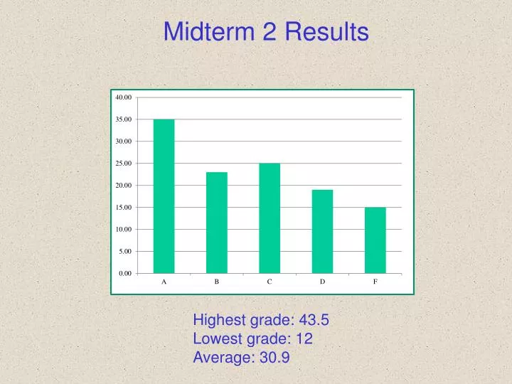
Midterm 2 Results Highest grade: 43.5 Lowest grade: 12 Average: 30.9
Greenhouse whitefly Parasitoid wasp A fly and its wasp predator: Laboratory experiment (Burnett 1959)
spider mite on its own with predator in simple habitat Spider mites with predator in complex habitat (Laboratory experiment) Predatory mite (Huffaker 1958)
Azuki bean weevil and parasitoid wasp (Laboratory experiment) (Utida 1957)
collared lemming stoat (Greenland) lemming stoat (Gilg et al. 2003)
Wood mouse (field observation: England) Tawny owl (Southern 1970)
prey boom predator boom Predator bust prey bust Possible outcomes of predator-prey interactions: • The predator goes extinct. • Both species go extinct. • Predator and prey cycle: • Predator and prey coexist in stable ratios.
Putting together the population dynamics: Predators (P): Victim consumption rate -> predator birth rate Constant predator death rate Victims (V): Victim consumption rate -> victim death rate Logistic growth in the absence of predators
Choices, choices…. • Victim growth assumption: • exponential • logistic • Functional response of the predator: • always proportional to victim density (Holling Type I) • Saturating (Holling Type II) • Saturating with threshold effects (Holling Type III)
The simplest predator-prey model (Lotka-Volterra predation model) Exponential victim growth in the absence of predators. Capture rate proportional to victim density (Holling Type I).
Predator density Victim isocline: Predator isocline: Victim density
Predator density Victim isocline: Predator isocline: Victim density dV/dt < 0 dP/dt < 0 dV/dt < 0 dP/dt > 0 dV/dt > 0 dP/dt > 0 dV/dt > 0 dP/dt < 0 Show me dynamics
Predator density Victim isocline: Predator isocline: Victim density
Predator density Victim isocline: Preator isocline: Victim density
Predator density Victim isocline: Preator isocline: Victim density Neutrally stable cycles! Every new starting point has its own cycle, except the equilibrium point. The equilibrium is also neutrally stable.
Logistic victim growth in the absence of predators. Capture rate proportional to victim density (Holling Type I).
r a r c Predator density Victim density Predator isocline: Victim isocline: Show me dynamics
P V Stable Point ! Predator and Prey cycle move towards the equilibrium with damping oscillations.
Exponential growth in the absence of predators. Capture rate Holling Type II (victim saturation).
r kD Predator density Victim density Victim isocline: Predator isocline: Show me dynamics
Unstable Equilibrium Point! Predator and prey move away from equilibrium with growing oscillations. P V
P V Unstable Equilibrium Point! Predator and prey move away from equilibrium with growing oscillations.
No density-dependence in either victim or prey (unrealistic model, but shows the propensity of PP systems to cycle): P V P Intraspecific competition in prey: (prey competition stabilizes PP dynamics) V P Intraspecific mutualism in prey (through a type II functional response): V
Predators population growth rate (with type II funct. resp.): Victim population growth rate (with type II funct. resp.):
Predator density Predator isocline: Victim isocline: Victim density Rosenzweig-MacArthur Model
Predator density Predator isocline: Victim isocline: Victim density Rosenzweig-MacArthur Model At high density, victim competition stabilizes: stable equilibrium!
Predator density Predator isocline: Victim isocline: Victim density Rosenzweig-MacArthur Model At low density, victim mutualism destabilizes: unstable equilibrium!
Predator density Predator isocline: Victim isocline: Victim density Rosenzweig-MacArthur Model At low density, victim mutualism destabilizes: unstable equilibrium! However, there is a stable PP cycle. Predator and prey still coexist!
The Rosenzweig-MacArthur Model illustrates how the variety of outcomes in Predator-Prey systems can come about: • Both predator and prey can go extinct if the predator is too efficient capturing prey (or the prey is too good at getting away). • The predator can go extinct while the prey survives, if the predator is not efficient enough: even with the prey is at carrying capacity, the predator cannot capture enough prey to persist. • With the capture efficiency in balance, predator and prey can coexist. • a) coexistence without cyclical dynamics, if the predator is relatively inefficient and prey remains close to carrying capacity. • b) coexistence with predator-prey cycles, if the predators are more efficient and regularly bring victim densities down below the level that predators need to maintain their population size.