Download
1 / 61
610 likes | 841 Views
Particle Systems on GPU. Youngho Kim CIS665: GPU Programming. Outline. Building a Million Particle System: Lutz Latta UberFlow - A GPU-based Particle Engine: Peter Kipfer et al. Real-Time Particle Systems on the GPU in Dynamic Environments: Shannon Drone

E N D
Particle Systems on GPU Youngho Kim CIS665: GPU Programming
Outline • Building a Million Particle System: Lutz Latta • UberFlow - A GPU-based Particle Engine: Peter Kipfer et al. • Real-Time Particle Systems on the GPU in Dynamic Environments: Shannon Drone • GPU-based Particle Systems for Illustrative Volume Rendering: R.F.P. van Pelt et al.
Sample Particle System Water Effects Nvdia DirectX10, Soft Particle
Building a Million Particle System: SIGGRAPH 2004 Lutz Latta
What is a particle system? One of the original uses was in the movie Star Trek II William Reeves (implementor) • Each Particle Had: • Position • Velocity • Color • Lifetime • Age • Shape • Size • Transparency Particle system from Star Trek II: Wrath of Khan
Old Game Examples Asteroids: 1978 Uses short moving vectors for Explosions Probably first “physical” particle simulation in CG/games Spacewar: 1962 Uses pixel clouds as Explosions Random motion
Types of Particle Systems • Stateless Particle System • A particle data is computed from birth to death by a closed form function defined by a set of start values and a current time. • Does not react to dynamic environment • Fast • State Preserving Particle System • Uses numerical iterative integration methods to compute particle data from previous values and changing environmental descriptions.
Stateless Particle System • Movie Clip
Stateless Particle Systems on GPU • Stateless Simulation – Computed particle data by closed form functions • No reaction on dynamically changing environment! • No Storage of varying data (sim. in vertex prog) Particle Birth Rendering Upload time of birth & initial Values to dynamic vertex buffer Set global function parameter as vertex program constants Render point sprites/triangles/quads With particle system vertex program
Particle Life Cycle • Generation – Particles are generated randomly within a predetermined location • Particle Dynamics – The attributes of a particle may vary over time. Based upon equations depending on attribute. • Extinction • Age – Time the particle has been alive • Lifetime – Maximum amount of time the particle can live. • Premature Extinction: • Running out of bounds • Hitting an object (ground) • Attribute reaches a threshold (particle becomes transparent)
Rendering • Rendered as a graphics primitive (blob) • Particles that map to the same pixels are additive • Sum the colors together • No hidden surface removal • Motion blur is rendered by streaking based on the particles position and velocity
Issues with Particle Systems on the CPU • CPU based particle systems are limited to about 10,000 particles per frame in most game applications • Limiting Factor is CPU-GPU communication • PCI Express transfer rate is about 3 gigabytes/sec
State Preserving Algorithm: Rendering Passes: • Process Birth and Deaths • Update Velocities • Update Positions • Sort Particles (optional, takes multiple passes) • Transfer particle positions from pixel to vertex memory • Render particles
Data Storage: • Two Textures (position and velocity) • Each holds an x,y,z component • Conceptually a 1d array • Stored in a 2d texture • Use texture pair and double buffering to compute new data from previous data • Storage Types • Velocity can be stored using 16bit floats • Size, Color, Opacity, etc. • Simple attributes, can be added later, usually computed using the stateless method
Birth and Death • Birth = allocation of a particle • Associate new data with an available index in the attributes textures • Serial process – offloaded to CPU • Initial particle data determined on CPU also • Death = deallocation of a particle • Must be processed on CPU and GPU • CPU – frees the index associated with particle • GPU – extra pass to move any dead particles to unseen areas (i.e. infinity, or behind the camera) • In practice particles fade out or fall out of view (Clean-up rarely needs to be done)
Allocation on CPU Stack Heap 2 5 2 10 5 30 10 15 11 30 6 15 26 19 12 26 33 11 19 Optimize heap to always return smallest available index 12 6 33 Better! Easier!
Update Velocities Velocity Operations • Global Forces • Wind • Gravity • Local Forces • Attraction • Repulsion • Velocity Damping • Collision Detection F = Σ f0 ... fn F = ma a = F/m If m = 1 F = a
Local Force – Flow Field Stokes Law of drag force on a sphere Fd = 6Πηr(v-vfl) η = viscosity r = radius of sphere C = 6Πηr (constant) v = particle velocity vfl = flow velocity Sample Flow Field
Other velocity operations • Damping • Imitates viscous materials or air resistance • Implement by downward scaling velocity • Un-damping • Self-propelled objects (bee swarms) • Implement by upward scaling velocity
Collisions • Collisions against simple objects • Walls • Bounding Spheres • Collision against complex objects • Terrain • Complex objects • Terrain is usually modeled as a texture-based height field
Collision Reaction vn = (vbc * n)vbc vt = vbc – vn vbc = velocity before collision vn = normal component of velocity vt = tangental component of velocity V = (1-μ)vt – εvn μ = dynamic friction (affects tangent velocity) ε = resilience (affects normal velocity) Vn V Vt
Update Positions: Euler Integration • Integrate acceleration to velocity: • v = vp + a⋅ ∆ t • Integrate velocity to position: • p= pp + v⋅ ∆ t • Computationally simple • Needs storage of particle position and velocity
Update Positions: Verlet Integration • Integrate acceleration to position: • p = 2pp − ppp a⋅t2 • ppp: position two time steps before • Needs no storage of particle velocity • Time step needs to be (almost) constant • Explicit manipulations of velocity (e.g. for collision) impossible
Sorting for Alpha Blending • Odd-even merge sort • Good for GPU because it always runs in constant time for a given data size • Inefficient to check whether sort is done on GPU • Guarantees that with each iteration sortedness never decreases • Full sort can be distributed over 20-50 frames so it doesn’t slow down system too much (acceptable visual errors)
UberFlow A GPU-based Particle Engine: SIGGRAPH 2004 Peter Kipfer et al.
Motivation • Major bottleneck • Transfer of geometry to graphics card • Process on GPU if transfer is to be avoided • Need to avoid intermediate read-back also • Requires dedicated GPU implementations • Perform geometry handling for rendering on GPU
GPU particle engine features • Particle advection • Motion according to external forces and 3D force field • Sorting • Depth-test and transparent rendering • Spatial relations for collision detection • Rendering • Individually colored points • Point sprites
Particle Advection • Simple two-pass method using two vertex arrays in double-buffer mode • Render quad covering entire buffer • Apply forces in fragment shader Buffer 0 Render target Bind to texture Screen Pass 1: integrate Buffer 1 Bind to render target Pass 2: render Bind to vertex array
Particle-Scene Collision • Additional buffers for state-full particles • Store velocity per particle (Euler integration) • Keep last two positions (Verlet integration) • Simple: Collision with height-field stored as 2D • texture • RGB = [x,y,z] surface normal • A = [w] height • Compute reflection vector • Force particle to field height
Particle – Particle Collision • Essential for natural behavior • Full search is O(n²), not practicable • Approximate solution by considering only neighbors • Sort particles into spatial structure • Staggered grid misses only few combinations
Particle – Particle Collision • Check m neighbors to the left/right • Collision resolution with first collider (time sequential) • Only if velocity is not excessively larger than integration step size
Real-Time Particle Systems on the GPU in Dynamic Environments: SIGGRAPH 2007 Shannon Drone
Non-parametric GPU particle systems • Storage requirements • Integrating the equations of motion • Saving particle states • Changing behaviors
Storage requirements • Need to store immediate particle state (position, velocity, etc) • Option 1: Store this data in a vertex buffer • Each vertex represents the immediate state of the particle • Particles are store linearly in the buffer • Option 2: Store this data in a floating point texture array • First array slice stores positions for all particles. • Next array slice stores velocities, etc.
Integrating the equations of motion • Accuracy depends on the length of time step • Use Euler integration for these samples • Runge-Kutta based schemes can be more accurate at the expense of needing to store more particle state
Saving particle states • Integration on the CPU can use read-modify-write operations to update the state in-place • This is illegal on the GPU (except for nonprogramming blending hardware) • Use double buffering • Ping-pong between them
Changing behaviors • Particles are no longer affixed to a predestined path of motion as in parametric systems • Changing an individual velocity or position will change the behavior of that particle. • This is the basis of every technique in this theory
Particles that react to other particles • N-Body problems • Force splatting for N2 interactions • Gravity simulation • Flocking particles on the GPU
N-Body problems • Every part of the system has the possibility of affecting every other part of the system • Space partitioning can help • Treating multiple parts of a system at a distance as one individual part can also help • Parallelization can also help (GPU)
Force splatting for N2 interactions • Our goal is to project the force from one particle onto all other particles in the system • Create a texture buffer large enough to hold forces for all particles in the simulation • Each texel holds the accumulated forces acting upon a single particle
Force splatting by rendering multiple into a force texture with alpha blending • It is O(N2), but it exploits the fast rasterization, blending, and SIMD hardware of the GPU • It also avoids the need to create any space partitioning structures on the GPU
Gravity simulation • Uses force splatting to project the gravitational attraction of each particle onto every other particle • Handled on the GPU • CPU only sends time-step information to the GPU • CPU also handles high-level switching of render targets and issuing draw calls
Flocking particles on the GPU • Uses basic boids behaviors • [Reynolds87,Reynolds99] to simulation thousands of flocking spaceships on the GPU • Avoidance • Separation • Cohesion • Alignment
Flocking particles on the GPU • Cohesion and Alignment • Unlike N-Body problems, Cohesion and Alignment need the average of all particle states • Cohesion steers ships toward the common center. • Alignment steers ships toward the common velocity • We could average all of the positions and velocities by repeatedly down-sampling the particle state buffer / texture • However, the graphics system can do this for us
Flocking particles on the GPU • Graphics infrastructure can already perform this quick down-sampling by generating mip maps • The smallest mip in the chain is the average of all values in the original texture
Reacting to arbitrary objects using RTV • Extend 2D partitioned grid [Lutz04] to 3D by rendering the scene into a volume texture • Instance the geometry across all slices • For each instance we clip the geometry to the slice • For each voxel in the volume texture stores the plane equation and velocity of the scene primitive
Painting with particles using gather • Once having the position buffer, it can gather paint splotches • Use a gather pixel shader to traverse the position buffer • For each particle in the buffer, the shader samples its position and determines if it can affect the current position in the position buffer • If it can, the color of the particle is sent to the output render target, which doubles as the mesh texture