Download

1 / 48
480 likes | 600 Views
Biostat Review. November 29, 2012. Objectives. Review hw#8 Review of last two lectures Linear regression Simple and multiple Logistic regression. Review hw#8. Simple linear regression.

E N D
Biostat Review November 29, 2012
Objectives • Review hw#8 • Review of last two lectures • Linear regression • Simple and multiple • Logistic regression
Simple linear regression • The objective of regression analysis is to predict or estimate the value of the response(outcome) that is associated with a fixed value of the explanatory variable (predictor).
Simple linear regression • The regression line equation is • The “best” line is the one that finds the α and β that minimize the sum of the squared residuals Σei2 (hence the name “least squares”) • We are minimizing the sum of the squares of the residuals • The slope is the change in the mean value of y that corresponds to a one-unit increase in x
Assumptions of the linear model • conditional mean of the outcome is linear • observed outcomes are independent • residuals (ε) follow a standard normal distribution • constant variance (σ2) • predictors are measured without error
Simple linear regression example: Regression of age on FEVFEV= α̂ + β̂ age regress yvarxvar . regress fev age Source | SS df MS Number of obs = 654 -------------+------------------------------ F( 1, 652) = 872.18 Model | 280.919154 1 280.919154 Prob > F = 0.0000 Residual | 210.000679 652 .322086931 R-squared = 0.5722 -------------+------------------------------ Adj R-squared = 0.5716 Total | 490.919833 653 .751791475 Root MSE = .56753 ------------------------------------------------------------------------------ fev | Coef. Std. Err. t P>|t| [95% Conf. Interval] -------------+---------------------------------------------------------------- age | .222041 .0075185 29.53 0.000 .2072777 .2368043 _cons | .4316481 .0778954 5.54 0.000 .278692 .5846042 ------------------------------------------------------------------------------ β̂ ̂ = Coef for age α̂ = _cons (short for constant)
Interpretation of coefficients β̂ ̂ = Coef. for age • For every one increase unit in age there is an increase in mean FEV of 0.22 α̂ = _cons (short for constant) • When age = 0, the mean FEV is 0.431, which is also equal to the mean FEV
Model Fit • R2 represents the portion of the variability that is removed by performing the regression on X • Remember that the R2 square tells us the fit of the model with values closer to 1 having a better fit
regress fev age Source | SS df MS Number of obs = 654 -------------+------------------------------ F( 1, 652) = 872.18 Model | 280.919154 1 280.919154 Prob > F = 0.0000 Residual | 210.000679 652 .322086931 R-squared = 0.5722 -------------+------------------------------ Adj R-squared = 0.5716 Total | 490.919833 653 .751791475 Root MSE = .56753 ------------------------------------------------------------------------------ fev | Coef. Std. Err. t P>|t| [95% Conf. Interval] -------------+---------------------------------------------------------------- age | .222041 .0075185 29.53 0.000 .2072777 .2368043 _cons | .4316481 .0778954 5.54 0.000 .278692 .5846042 ------------------------------------------------------------------------------ =.75652
Model fit • Residuals are the difference between the observed y values and the regression line for each value of x ( yi-ŷi) • If all the points lie along a straight line, the residuals are all 0 • If there is a lot of variability at each level of x, the residuals are large • The sum of the squared residuals is what was minimized in the least squares method of fitting the line
Use of residual plots for model fit • Residual plot is a scatter plot • Y-axis residuals • X-axis outcome variable • Stata code to get residual plot: regress fev age rvfplot
rvfplot, title(Fitted values versus residuals for regression of FEV on age)
Why look at residual plot • The spread of the residuals increase s with fitted in FEV values increases,– suggesting heteroscedasticity • Heteroscedasticityreduces the precision of the estimates (hence reduces power) -makes your standard errors larger • Homoscedasticity: constant variability across all values of x (same standard deviation for each value of y) -constant variance (σ2) assumption
Residual plots • Of note • rvfplot ** gives you Residuals vs. Fitted (outcome) • rvpplotht ** gives you Residuals vs. Predictor (predictor)
Data transformation • So if you have heterostatisticity in your data, can transform your data • Something to note • Transforming you data does not inherently change your data • Log transformation is the most common way to deal with heterostatisticity
Log transformation of FEV data • Do we still have heterostatisticity?
Log transformation stata output . regress ln_fev age Source | SS df MS Number of obs = 654 -------------+------------------------------ F( 1, 652) = 961.01 Model | 43.2100544 1 43.2100544 Prob > F = 0.0000 Residual | 29.3158601 652 .044962976 R-squared = 0.5958 -------------+------------------------------ Adj R-squared = 0.5952 Total | 72.5259145 653 .111065719 Root MSE = .21204 ------------------------------------------------------------------------------ ln_fev | Coef. Std. Err. t P>|t| [95% Conf. Interval] -------------+---------------------------------------------------------------- age | .0870833 .0028091 31.00 0.000 .0815673 .0925993 _cons | .050596 .029104 1.74 0.083 -.0065529 .1077449 -------------------------------------------------------------
Interpretation of regression coefficients for transformed y value • The regression equation is: ln(FEV) = ̂ + ̂ age = 0.051 + 0.087 age • So a one year change in age corresponds to a .087 change in ln(FEV) • The change is on a multiplicative scale, so if you exponentiate, you get a percent change in y • e0.087 = 1.09 – so a one year change in age corresponds to a 9% increase in FEV
Categorical variable/predictor • Previous example was of a predictor that was continuous • Can also perform regression with a categorical predictor/variable • If dichotomous • Convention use 0 vs. 1 • ie is dichotomous: 0 for female, 1 for male
Categorical independent variable • Remember that the regression equation is μy|x = α + x • The only variables x can take are 0 and 1 • μy|0 = αμy|1 = α + • So the estimated mean FEV for females is ̂ and the estimated mean FEV for males is ̂ + ̂ • When we conduct the null hypothesis test that=0 • Similar to a -T-test
Categorical variable/predictor • What if you have more than two categories within a predictor (non-dichotomous)? • One is set to be the reference category.
Categorical independent variables • Then the regression equation is: y = + 1 xAsian/PI + 2 xOther+ ε • For race group= White (reference) ŷ = ̂ +v ̂10+ ̂20 = ̂ • For race group= Asian/PI ŷ = ̂ + ̂11 + ̂20 = ̂ + ̂1 • For race group= Other ŷ = ̂ + ̂10 + ̂21 = ̂ + ̂2
Categorical independent variables • For stata you just place an “i.variable” to identify it as categorical variable • Stata takes the lowest number as the reference group • You can change this by the prefix “b#. variable” where # is the number value of the group that you want to be the reference group.
Multiple regression • Additional explanatory variables might add to our understanding of a dependent variable • We can posit the population equation μy|x1,x2,...,xq = α + 1x1 + 2x2 + ... + qxq • αis the mean of y when all the explanatory variables are 0 • iis the change in the mean value of y the corresponds to a 1 unit change in xiwhen all the other explanatory variables are held constant
Multiple regression • Stata command (just add the additional predictors) • regress outcomevar predictorvar1 predictorvar2…
Multiple regression . regress fev age ht Source | SS df MS Number of obs = 654 -------------+------------------------------ F( 2, 651) = 1067.96 Model | 376.244941 2 188.122471 Prob > F = 0.0000 Residual | 114.674892 651 .176151908 R-squared = 0.7664 -------------+------------------------------ Adj R-squared = 0.7657 Total | 490.919833 653 .751791475 Root MSE = .4197 ------------------------------------------------------------------------------ fev | Coef. Std. Err. t P>|t| [95% Conf. Interval] -------------+---------------------------------------------------------------- age | .0542807 .0091061 5.96 0.000 .0363998 .0721616 ht | .1097118 .0047162 23.26 0.000 .100451 .1189726 _cons | -4.610466 .2242706 -20.56 0.000 -5.050847 -4.170085 ------------------------------------------------------------------------------ • R2 will always increase as you add more variables into the model • The Adj R-squared accounts for the addition of variables and is comparable across models with different numbers of parameters • Note that the beta for age decreased
How do you interpret the coefficients? • Age • Whenheight is held constant for every 1 unit (in this case year) increase in age you will have a 0.054 unit increase in FEV
You can fit both continuous and categorical predictors . regress fev age smoke Source | SS df MS Number of obs = 654 -------------+------------------------------ F( 2, 651) = 443.25 Model | 283.058247 2 141.529123 Prob > F = 0.0000 Residual | 207.861587 651 .319295832 R-squared = 0.5766 -------------+------------------------------ Adj R-squared = 0.5753 Total | 490.919833 653 .751791475 Root MSE = .56506 ------------------------------------------------------------------------------ fev | Coef. Std. Err. t P>|t| [95% Conf. Interval] -------------+---------------------------------------------------------------- age | .2306046 .0081844 28.18 0.000 .2145336 .2466755 smoke | -.2089949 .0807453 -2.59 0.010 -.3675476 -.0504421 _cons | .3673731 .0814357 4.51 0.000 .2074647 .5272814 ------------------------------------------------------------------------------ • The model is fêv = α̂ + β̂1 age + β̂2Xsmoke • So for non-smokers, we have fêv= α̂ + β̂1 age (b/c Xsmoke=0) • For smokers, fêv = α̂ + β̂1 age + β̂2(b/c Xsmoke= 1) • So β̂2 is the mean difference in FEV for smokers versus non-smokers at each age
When you have one continuous variable and one dichotomous variable, you can think of fitting two lines that only differ in y intercept by the coefficient of the dichotomous variable (in this case smoke) • E.g. β̂2=-.209
Linear regression summary • Intercept is the mean value of outcome for an individual with other values equal to zero • Mean change in the outcome per unit change in the predictor • Mean change in the outcome per unit change in predictor holding other variables constant • R-squared is the proportion of total variance in the outcome explained by the regression model • Adjusted R-squared accounts for the number of predictors in the model
Logistic regression • Linear regression • Continuous outcome • Logistic regression • Dichotomous outcome • Eg disease or no disease or Alive/Dead • Model the probability of the disease
Logistic regression • Need an equation that will follow rules of probability • Specifically that probability needs to be between 0-1 • A model of the form p= α + βx would be able to take on negative values or values more than 1 • p=e α + βx is an improvement because it cannot be negative , but it still could be greater than 1
Logistic regression • How about the function? • This function =.5 when α + βx =0 • The function models the probability slowly increasing over the value of x, until there is a steep rise, and another leveling off
Logistic regression • ln(p/(1-p)) = α + bx • So instead of assuming that the relationship between x and p is linear , we are assuming that the relationship between ln(p/(1-p)) and x is linear. • ln(p/(1-p)) is called the logit function • It is a transformation • While the outcome is not linear, the other side of the equation α + bx is linear
Logistic regression • Stata code • logistic outcomevarpredictorvar 1 predictorvar2…, coef • Coef command gives you coefficient, β • This β, when you are interpreting is actually ln(OR) • To get the odds ratio, need to raise β to e • Odds ratio = e • Or you could just use this stata code instead (don’t use coeff) • logistic outcomevarpredictorvar 1 predictorvar2…,
Interpret these coefficients . logistic coldany i.rested_mostly, coef Logistic regression Number of obs = 504 LR chi2(1) = 19.71 Prob > chi2 = 0.0000 Log likelihood = -323.5717 Pseudo R2 = 0.0296 ------------------------------------------------------------------------------ coldany | Coef. Std. Err. z P>|z| [95% Conf. Interval] -------------+---------------------------------------------------------------- 1.rested_m~y | -.9343999 .2187794 -4.27 0.000 -1.3632 -.5056001 _cons | -.2527658 .1077594 -2.35 0.019 -.4639704 -.0415612 ------------------------------------------------------------------------------
Interpret these coefficients • Cold data (from previous slide) • β = -0.934 • The natural log of the odds of someone who was rested of getting a cold to someone who is rested is -0.934 • If you raise it to the power of e, you get 0.39 • Therefore another way of interpreting this is that the odds of someone who was rested of getting a cold compared to someone who is not rested is 0.39
Or get stata to calculate the odds ratio for you! logistic depvarindepvar . logistic coldanyi.rested_mostly Logistic regression Number of obs = 504 LR chi2(1) = 19.71 Prob > chi2 = 0.0000 Log likelihood = -323.5717 Pseudo R2 = 0.0296 ------------------------------------------------------------------------------ coldany | Odds Ratio Std. Err. z P>|z| [95% Conf. Interval] -------------+---------------------------------------------------------------- 1.rested_m~y | .3928215 .0859413 -4.27 0.000 .2558409 .6031435 ------------------------------------------------------------------------------ =e
Interpretation when you have a continuous variable . . logistic coldany age Logistic regression Number of obs = 504 LR chi2(1) = 23.77 Prob > chi2 = 0.0000 Log likelihood = -322.05172 Pseudo R2 = 0.0356 ------------------------------------------------------------------------------ coldany | Odds Ratio Std. Err. z P>|z| [95% Conf. Interval] -------------+---------------------------------------------------------------- age | .9624413 .0081519 -4.52 0.000 .9465958 .9785521 ------------------------------------------------------------------------------ • Interpretation of the coefficients: The odds ratio is for a one unit change in the predictor • For this example the 0.962 is the odds ratio for a year difference in age
Continuous explanatory variable • To find the OR for a 10-year change in age . . logistic coldany age, coef Logistic regression Number of obs = 504 LR chi2(1) = 23.77 Prob > chi2 = 0.0000 Log likelihood = -322.05172 Pseudo R2 = 0.0356 ------------------------------------------------------------------------------ coldany | Coef. Std. Err. z P>|z| [95% Conf. Interval] -------------+---------------------------------------------------------------- age | -.0382822 .00847 -4.52 0.000 -.0548831 -.0216813 _cons | .906605 .3167295 2.86 0.004 .2858265 1.527383 ------------------------------------------------------------------------------ OR for a 10-year change in age = exp(10*-.0382) = 0.682
Or you can also generate a new variable • To find the OR for a 10-year change in age . gen age_10=age/10 (2 missing values generated) . logistic coldany age_10 Logistic regression Number of obs = 504 LR chi2(1) = 23.77 Prob > chi2 = 0.0000 Log likelihood = -322.05172 Pseudo R2 = 0.0356 ------------------------------------------------------------------------------ coldany | Odds Ratio Std. Err. z P>|z| [95% Conf. Interval] -------------+---------------------------------------------------------------- age_10 | .6819344 .0577599 -4.52 0.000 .5776247 .8050807 ------------------------------------------------------------------------------ This is nice because stata will calculate your confidence interval as well!
Interpret this output . logistic coldany age_10 i.smoke Logistic regression Number of obs = 504 LR chi2(2) = 23.89 Prob > chi2 = 0.0000 Log likelihood = -321.99014 Pseudo R2 = 0.0358 ------------------------------------------------------------------------------ coldany | Odds Ratio Std. Err. z P>|z| [95% Conf. Interval] -------------+---------------------------------------------------------------- age_10 | .6835216 .0580647 -4.48 0.000 .5786864 .807349 1.smoke | 1.128027 .3863511 0.35 0.725 .5764767 2.20728 ------------------------------------------------------------------------------ .
Correct interpretations For this example the 0.684 is the odds ratio for a ten-year difference in age when you hold smoking status constant 1.13 is the odds ratio for smoking when you hold age constant
. logistic sex fev Logistic regression Number of obs = 654 LR chi2(1) = 29.18 Prob > chi2 = 0.0000 Log likelihood = -438.47993 Pseudo R2 = 0.0322 ------------------------------------------------------------------------------ sex | Odds Ratio Std. Err. z P>|z| [95% Conf. Interval] -------------+---------------------------------------------------------------- fev | 1.660774 .1617468 5.21 0.000 1.372176 2.01007 _cons | .279198 .0742534 -4.80 0.000 .1657805 .4702094 ------------------------------------------------------------------------------ the z (Wald) test statistic in the logistic results is the ratio of the estimated regression coefficient for the predictor (fev)to its standard error , and follows (approximately) a standard normal distribution the log-likelihood is a measure of support of the data for the model (the larger the likelihood and/or log-likelihood, the better the support). the statistic "chi2" is the likelihood ratio statistic for comparing this model including arcus to the simpler one (presented below) containing no predictors
Summary Logistic regression • The log-odds of the outcome is linear in x, with intercept αand slope β1 . • The "intercept" coefficient αgives the log-odds of the outcome for x = 0. • The "slope" coefficient β1 gives the change in log-odds of the outcome for a unit increase in x. This is the log odds ratio associated with a unit increase in x. • Outcome risk (P) is between 0 and 1 for all values of x