Download
1 / 27
270 likes | 406 Views
What is a balance sheet?. Shows the financial position of an enterprise at a given point in timeProvides information about what an enterprise owns(assets), owes (liabilities) and its value to its inverstors (share holders equity)Accounting equationAssets = Liabilities stockholders' equityMeasu

E N D
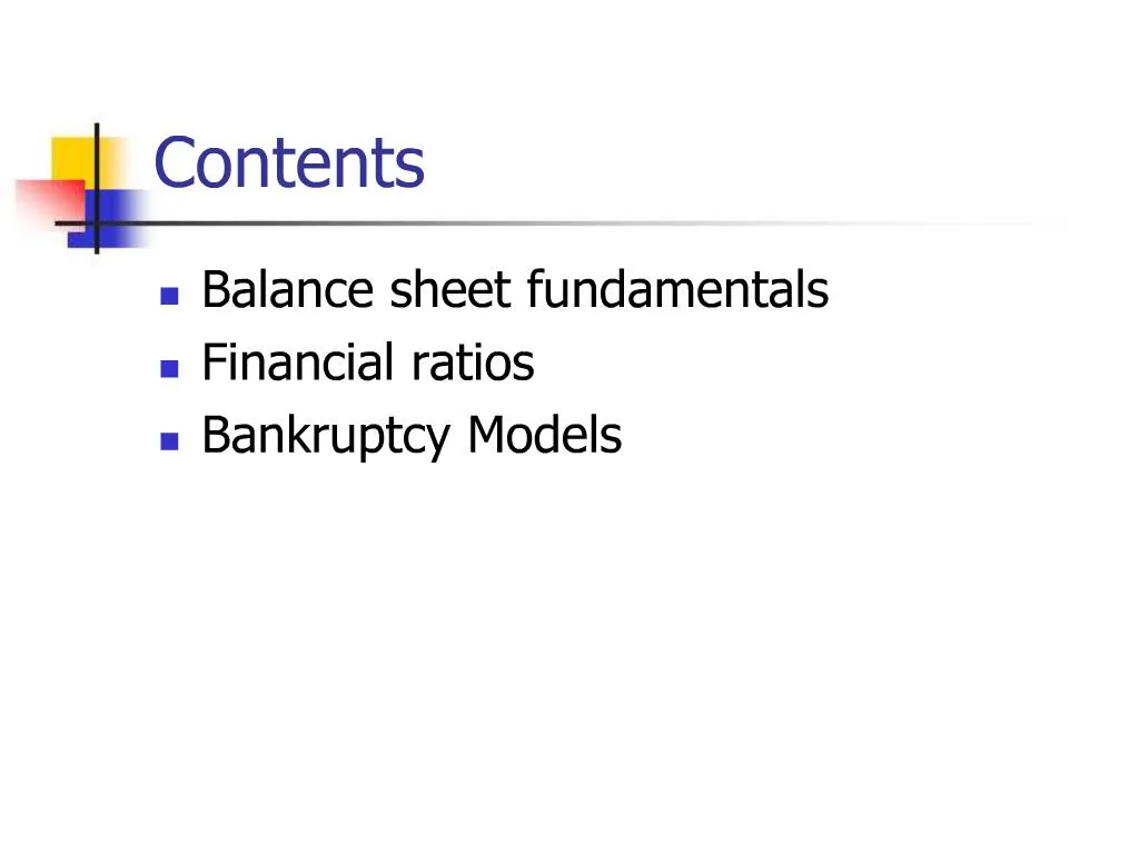
1. Contents Balance sheet fundamentals
Financial ratios
Bankruptcy Models
2. What is a balance sheet? Shows the financial position of an enterprise at a given point in time
Provides information about what an enterprise owns(assets), owes (liabilities) and its value to its inverstors (share holders equity)
Accounting equation
Assets = Liabilities + stockholders� equity
Measured at a point in time
3. Balance Sheet
4. Balance Sheet terminology Asset
Any item of economic value owned by a corporation
Liabilities
A financial claim, debt or potential loss that is owed by a corporation
Stockholder�s Equity
Value of the business a corporation generates that it owes to its shareholders after all its obligations have been met
5. Balance Sheet terminology Continued � Basic Accounts Equation
Asset = Liabilities + Shareholder�s equity
Owners Equity
Owners claim on the assets
Owners total investment
6. Prediction of Financial Distress Process of estimating the probability of the bankruptcy of a corporation by using financial ratios and existing models.
7. Models used in the prediction of financial distress Z-Score Model
Vasicek-Kealhofer model
Black- Scholes �Merton Probability
Compensator Model
8. The Z-score Model First developed by Altman in 1968
Uses a specified set of financial ratios as variables in multidiscriminant statistical methodology (MDR)
Real world application of the Altman score successfully predicted 72% of bankruptcies 2 years prior to their filing for Chapter 7
9. Multi Discriminant Analysis Used to classify an observation into several groupings
The groupings are based on an observation�s individual characteristics
MDR is used while making predications in problems where the variable dependant variable appears in qualitative form. Eg. Bankrupt and non-bankrupt
Forms a linear equation using characteristics that can be used to distinguish between the dependant variable groups
10. Z-score model :reprise Uses five financial ratios
Ratios are objectively weighed and summed
Ratios can be obtained from corporations financial statements
11. Z-score constituent ratios Working Capital/total assets (WC/TA)
Working Capital is the difference between the current assets and current liabilities as obtained from the balance sheet
Retained Earnings/total assets ( RE/TA)
Retained Earning is also know as the earned surplus
It represents the total amount of reinvested earnings and/or losses of a firm over its entire life-cyle
Can be obtained from balance sheet
Earnings before interest and taxes/Total assets (EBIT/TA)
Measure of a corporation�s earning power from ongoing operations
Also know as Operating profit
Watched closely by creditors as it represent the total amount of cash that a corporation can use to pay off its creditors
Can be obtained for the Income statement
12. Z-score constituent ratios Continued� Market Value of Equity/Book Value of total liabilities (MVE/TL)
The market value of equity is the total market value of all of the stock, both preferred and common
The book value of liabilities is the total value of liabilities both long term and current
The MVE/TL shows how much the firms assets can decline in value with increasing liabilities, before the liabilities exceed the assets
Sales/Total Assets (s/TA)
Also known as capital turnover ratio
Illustrates the sales generating ability of the corporation�s assets
13. Z score Results Based on Z-scores averaged over time, Altman calculated that a Z-score <2.675 could be classified as failed
More accurately, Z<1.81 signals bankruptcy within 1 year
Z > 2.99 signals the firm is in good financial health
14. VK model Uses EDF (expected default frequency) credit measures � the probability that a company will default within a given timeframe
3 main elements are used to determine the default probability
Market Value of assets
Asset Risk
Leverage � Extent of the corporation�s contractual liabilities. It is the book value of liabilities relative to the market value of assets
15. Leverage Default risk increases as the market value of the assets approaches the book value of the liabilities.
16. Market net worth Market net worth is market value of the company�s assets minus the default point
Market net worth is considered in context of the business risk
Food and beverage industries can afford higher leverage( lower market net worth) than technology businesses because their asset values are more stable
17. Asset Volatility It is the standard deviation of the annual percentage change in the asset value
It is related to the size and nature of the industry
It can be calculated from the value of the increase or decrease in percentage of asset value upon 1 standard deviation change in the asset value
18. Distance to Default
19. Distance to Default Compares the market net worth to the size of a 1 standard deviation move in the asset value
Combines 3 key credit issues:
Value of firm�s assets
Business and industry risk
leverage
20. Determining Default Probability 3 steps to determine default probability
Estimate Asset value and volatility:
Equity is a call option on asset value. Equity holders have the right but are not obligated to pay off the debt holders
Solve for implied asset value and volatility
Calculate Distance to default:
Contractual obligations determine Default Point
Number of standard deviations from default
Calculate Default probabilty:
Assign EDF using actual historical rates
21. Black-Sholes-Merton Probability Volatility is crucial variable in bankruptcy prediction since it captures the likelihood that the values of firms assets will decline to such an extent that the firm will be unable to repay its debts
Equity can be viewed as a call option on the value of the firm�s assets. The strike price of the call option is equal to the face value of the firm�s liabilities and the option expires at time T when the debt matures.
The BSM equation:
Where N(d1) and N(d2) are the standard cumulative normal of d1 and d2 and
22.
VE is the current market value of equity; VA is the current market value of assets; X is the face value of debt maturing at time T; r is the continuously-compounded risk-free rate; d is the continuous dividend rate expressed in terms of VA and ?A is the std deviation of asset returns.
Under the BSM model . The probability of bankruptcy is simply the prob that the market value of assets , VA is less than the face value of the liabilities, X, at time T (i.e VA(T) < X). The BSM model assumes that the natural log of future asset values is distributed normally as follows, where u is the continuously compounded expected return on assets:
23. The probability that VA(T) < X is as follows:
This shows the prob of bankruptcy is a function of the distance btw the current value of the firm�s assets and the face value of the liabilities adjusted for the expected growth in asset values
relative to the asset volatility
We must estimate the market value of assets, asset volatility and the expected return on assets.
We estimate the values of VA and by simultaneously solving the call option equation and the optimal hedge eqn :
We solve the two equations simultaneously for the two unknown variables VA and .The starting values are determined by setting VA equal to book value of liabilities plus market value of equity and
In the second step, we estimate the expected market return on assets, u, based on the actual return on assets during the previous year, based on the estimates of VA that were computed in the previous step.
24.
Finally we use these values to calculate the BSM-Prob for each firm year.
25. Compensator Model Based on the assumption of incomplete information : bond investors are not certain abut the true level of firm value that will trigger default. Coherent integration of structure and uncertainty is facilitated with compensators.
In reality, default, or at least the moment at which default is publicly known to be inevitable , usually comes as a surprise. Highlighted in credit market by the prevalence of positive short-term credit spreads.
Features :
Structure plus uncertainty � integrate an intuitive, cause-and-effect model with the uncertainty that surrounds default events
Economic reasonability and flexibility
Unified perspective � broad enough to incorporate intensity based models and traditional structural models
For t>0 let F(t) be the prob of default before time t. If G(w) is the time of default in state w, then F(t) = P[G(w)<=t] which is strictly < 1.
Consider the function: A(t) = -log(1-F(t)) . This is called the pricing trend of the default process. The pricing trend can be analyzed directly with the mathematical theory of compensators:
The difference btw an underlying process and its compensator is a martingale
The compensator is non decreasing
Compensator is predictable even if underlying process is not
26. The compensator of the default process is continuous iff the default is completely unpredictable.
Compensators, and thus pricing trends depend both on the underlying structure that keeps track of the information acquired as time passes.
How to create compensators without the information structure? � use info generated by underlying process � survival information structure
Theory can be reworked with an eye to information available � histories of equity prices, debt outstanding , agency ratings and accounting variables. � Use this information to derive a pricing trend from which default probability can be estimated.
Now we have the conditional probability of default by time t, given info at time t as F(t,w), which gives the pricing trend as A(t,w) = -log(1-F(t,w))
F(t) = 1 - E[exp(-A(t,w)]
Alternatively, F(t) = E[F(t,w)]
27. Model specification:
Default triggered when the value of firm falls below barrier
Default barrier is not publicly known
The firm value process is given by a geometric Brownian motion
History of fundamental data and other publicly available info used to model the default barrier and firm value process