Download
1 / 80
800 likes | 1.04k Views
Market Equilibrium and Market Demand: Imperfect Competition. Chapter 9. Market Structure Characteristics. We characterize an industry by The number of firms and their size distribution Product differentiation Barriers to entry The picture to the right concerned with two markets:

E N D
MarketEquilibrium and Market Demand:Imperfect Competition Chapter 9
Market Structure Characteristics We characterize an industry by • The number of firms and their size distribution • Product differentiation • Barriers to entry • The picture to the right concerned with two markets: • No. 2 yellow corn: many producers/sellers (Perfect Competition) • Farm equipment: few manufacturers/sellers (Oligopoly) 2 Pages 145-148
Perfect Competition • Up to now we have been assuming the firm and market reflect conditions of perfect competition • Not a bad assumption for many agricultural subsectors • A large number of small firms: 2 million farms • A homogeneous product: No. 2 yellow corn • Freely mobile resources: No barriers to entry caused by patents, etc. or barriers to exit (???) • Perfect knowledge of market conditions: Quality outlook information from government, university and private sources 3
Imperfect Competition • Many markets in which farmers buy inputs and sell their products however do notreflect perfect competition conditions • Chapter 9 focuses on specific types of imperfect competitors in the farm input market • These firms are capable of setting prices farmers must pay for specific inputs 4
Topics for Nov 3rd • Monopolistic Competition • Definition • Production and Pricing Decisions • Oligopolies • Definition/Examples • Production and Pricing Decisions • Monopolies • Definition/Examples • Production and Pricing Decisions • Comparison of Market Structures Pages 106-107 6
Imperfect Competition in Selling • Unlike perfect competitors who face a perfectly elastic (horizontal) demand curve • Imperfect competitors selling a differentiated product have a downward sloping demand curve $ $ Firm’s demand curve under P.C. Firm’s demand curve under imperfect competition A A B B Q Q 7
Table 9-1 Imperfect Competition Firm faces a downward sloping demand curve → MR ≤ AR 2 20 Marginal Revenue (MR) : Change in revenue from the sale of the last unit of output (ΔTR÷ΔQ) Average Revenue (AR): Total Revenue/Total output (TR÷Q) Note: Price = Average Revenue 8 Page 149
Imperfect Competition in Selling Marginal Revenue: Change in revenue from the sale of the last unit of output 9 Page 150
Imperfect Competition in Selling Maximum Total Revenue • Marginal revenue in this instance is also downward sloping • MR=0 at the point where TR is at a maximum Page 150 10
Types of Imperfect Competitors in Input Markets • Monopolistic Competition • Oligopoly • Monopoly Let’s start here… 11
Monopolistic Competitors • Many sellers • Each firm has relatively small market share • Power to set prices somewhat like a monopoly • Face competition like perfect competition • Collusion is not possible given number of firms in the industry • No barriers to entry or exit 12 Page 148-151
Monopolistic Competitors • Product Differentiation: Each firm makes a product that is slightly different from the products of competing firms • Close substitutes but no perfect substitutes • An attempt to ↑ price will normally results in a ↓ in volume sold • Competition on Quality, Price, Marketing • Quality is design, reliability, service provided to buyer and ease of access to product • The firm faces a downward sloping demand curve • Firm must market intensively: promotions, distribution, packaging, etc. 13 Page 148-151
Monopolistic Competitors • Product differentiation does not necessarily mean there are any physical differences among products • They might all be the same, but how they are sold may make all the difference 14 Page 148-151
Monopolistic Competitors • The monopolistic competitor tries to set his/her product apart from the competition • Main method is via advertising • When this is done successfully, the demand curve becomes more vertical or inelastic • Buyers are willing to pay more because they believe it is much better than their other choices • Basis for product differentiation • Physical differences Convenience • Ambience Reputations • Appeals to vanity Snob appea 15 Page 148-151
Monopolistic Competitors • Typical Monopolistic Competitor • Tries to set firm apart from competition • New Product Development and Innovation • Advertising • Create consumer perception of product differentiation – real or imagined • Attempt to keep demand as inelastic as possible • Selling costs can be extremely high 16 Page 148-151
Monopolistic Competitors Short run profits can exist but long run profits are reduced to 0 with industry entrants Fast food industry is a good example All services basically the same Extensive use of marketing to differentiate products/services across firms Striving to produce more products and services 17 Page 148-151
Monopolistic Competitors Production Decision: Determine output level where MC=MR (Why does this make sense?) Pricing Decision: Determine where above quantity intersects the downward sloping demand curve 18 Page 148-151
Monopolistic Competition Short run profits exist if: PSR > ATCSR at QSR • Short run profits • The firm produces QSR where MR=MC at E • Prices its products at PSR by reading off the demand curve at quantity QSR • Represents consumer’s willingness to pay for QSR Page 150 19
Monopolistic Competition • Short run loss • At QSR, PSR < ATCSR Page 150 20
In the Long Run (LR) • Profits are bid away as more firms enter the market • Losses will no longer exist as firms leave the market • At QLR the remaining firms are just breaking even PLR = ATCLR Monopolistic Competition 21 Page 151
Monopolistic Competitors • How much is the industry dominated or not dominated by few suppliers • Geographical scope – national, regional, global • An industry can be almost perfectly competitive on a national scope, but almost a monopoly locally e.g. Feed Retailing • Barriers to entry and exit: industries may appear concentrated but few barriers exist to prevent entry 22 Page 148-151
Monopolistic Competitors • Quantitative measures of competition • Concentration Ratio (CR): 2,4, 8, 20, etc • % of the value of total market revenue accounted for by 2, 4, 8, 20, etc. largest firms in the industry • Low CR values→ a high degree of competition • High CR values → an absence of competition 23 Page 148-151
Monopolistic Competitors • Quantitative measures of competition • Herfindahl-Hirschman Index (HHI): The square of the % market share of each firm summed over the largest 50 firms in an industry or all firms if < 50 in industry • Perfect competition, HHI is small • Only 1 firm, HHI is 10,000 = (1002) • U.S. Justice Department • HHI < 1,000 competitive markets • HHI > 1,800 could be considered concentrated industry worthy of Justice Dept. examination of any purchases 24 Page 148-151
Oligopolies • A few number of sellers • Each can impact market price & quantities • Interdependent in their decision making • Key component in marketing strategies and pricing behavior • Match price cuts but not price increases by fellow oligopolists • Do this to maintain market share • Non-price competition between oligopolists to uniquely identify products 25 Pages 152-155
Oligopolies • Rival oligopolists will match price cuts but not price increases in the short run because they want to capture a larger market share • If there are differences in prices they are the result of successful product differentiation • Tend to have stable prices • Changes in production and other costs not easily passed on and may have to be absorbed 26 Pages 152-155
Oligopolies • Price leadership strategy • A particular firm dominates the market • Controls the largest share of the market • Other industry firms more efficient in operation, marketing, etc. • The dominant firm first sets its price to maximize profit • Remaining firms set their prices based on the dominant firms pricing • The price set by the oligopolist seller is higher under perfect competition • Quantity produced is lower then perfect comp. 27 Pages 152-155
Oligopolies • The dominant firm may be efficient enough to set a lower price • Eventually drive the other firms out of the market 28 Pages 152-155
Oligopolies • Examples of Oligopolies • Auto manufacturers • 1997 CR4 value of 97.4 • Aircraft manufacturing • Farm machinery and equipment • John Deere, J.I.Case and New Holland • 80% of 2-wheel drive tractors • close to 90% of combines sold in the U.S. • Cattle slaughtering • CR4 value increased from 39% to 67% over the 1985-1995 period 29 Pages 152-155
Demand curve DD • All oligopolists move prices together and share market • Demand curve dd • A singlefirm changes its price • Curve DD is more inelastic • Below point 1, firms match price cut • This leads to a kinked demand curve d1D • Leads to a discontinuous marginal revenue curve, d256 6 Remember oligopolists account for the reaction of other firms so there is no single demand curve 30 Page 154
Meeting demand along the lower segment of the kinked demand curve → the firm is maintaining its market share Page 154 31
Shifting MC curves reflecting technological advances will not affect PE and QE • It does impact profits as MC drops from pt 3 to pt 4 Page 154 32
Monopolies • One seller in the market • Entry of other firms restricted by patents, etc. (i.e., barrier to entry) • Firm has absolute power over setting market price • Produces a unique product • It can have economic profits in the long run because it can set price without competition 33 Page 155-156
Monopolies $/unit • Total revenue = area 0PECQE • Monopolist produces quantity where MC=MR (pt A), QE • Uses the demand curve (pt C) when setting price PE ATC MC AVC C PE B M A N Demand= AR TVC MR Quantity 0 QE 34 Page 155-156
Monopolies $/unit ATC MC AVC • Total variable costs for the monopolist is equal to area 0NAQE, (green box) • =AVC x QE = 0N x QE C PE B M A N Demand= AR TVC MR Quantity 0 QE 35 Page 155-156
Monopolies $/unit ATC MC AVC C PE • Total fixed costs equals NMBA (orange box) • =(ATC-AVC) x QE B M TFC A N Demand= AR MR Quantity 0 QE 36 Page 155-156
Monopolies $/unit ATC MC AVC • Total cost is area 0MBQE (green box + orange box) • = area ONAQE + area NMBA C PE B M TFC N A Demand= AR TVC MR Quantity 0 QE 37 Page 155-156
Monopolies $/unit Economic Profit ATC MC AVC C • Monopoly economic profit = area MPECB • = Total Revenue (yellow box) – Total Costs (green box + orange box) PE B M TFC A N Demand= AR TVC MR Quantity 0 QE 38 Page 155-156
Monopolies $/unit ATC MC AVC C PE Economic Profit • Total fixed costs equals NMBA (orange box) • =(ATC-AVC) x QE B M TFC A N Demand= AR TVC MR Quantity 0 QE 39 Page 155-156
Comparison of Structure Results • Lets compare the results we have obtained from the alternative market structures 40
Perfect Competition Case Consumer surplus = sum of areas 1, 4, 5, 8 and 9 (blue triangle) 41 Page 157
Perfect Competition Case • Producer surplus = to the sum of areas 2, 3, 6 and 7 (green triangle) Page 157 42
Perfect Competition Case • Total economic surplus = sum of blue and green triangles • =sum of areas 1 – 9 Page 157 43
CS = sum of areas 8 and 9, (new blue triangle) • Compared to P.C., consumers would be economically worse-off by areas 1, 4 and 5 • Paying a higher price, PM • Purchasing a smaller quantity, QM Monopoly Case Page 157 44
PS = to sum of areas 3, 4, 5, 6 and 7 (green area) • Compared to P.C. producers lose area 2 but gain areas 4 + 5 • Economically better-off than P.C. Monopoly Case Page 157 45
Society as a whole would be economically worse-off by areas 1+2 • Known as the dead weight loss • Reflects the fact that less of available resources in this market are used to provide products to consumers Monopoly Case 46 Page 157
Summary of Imperfect Competitors from a Selling Perspective Page 157 47
Types of Imperfect Competitors on the Buying Side • Monopsonistic competition • Oligopsony • Monopsony Let’s start here… 49
Monopsonies • Single buyer in the input market • Focus is on the marginal input cost of purchasing an addition unit of resources • Will purchase input until Marginal Value Product (MVP)=Marginal Input Cost (MIC) • As long as MVP>MIC, the monopsonist makes a profit 50 Page 158-160