Download
1 / 35
360 likes | 446 Views
Understand how to estimate unknown densities with parameter estimation techniques like Maximum Likelihood and Bayesian Estimation. Learn about Bias-Variance Decomposition and Model Selection procedures to balance the trade-off in model complexity.

E N D
Bias and Variance of the Estimator PRML 3.2 Ethem Chp. 4
In previous lectures we showed how to build classifiers when the underlying densities are known • Bayesian Decision Theory introduced the general formulation • In most situations, however, the true distributions are unknown and must be estimated from data. • Parameter Estimation (we saw the Maximum Likelihood Method) • Assume a particular form for the density (e.g. Gaussian), so only the parameters (e.g., mean and variance) need to be estimated • Maximum Likelihood • Bayesian Estimation • Non-parametric Density Estimation(not covered) • Assume NO knowledge about the density • Kernel Density Estimation • Nearest Neighbor Rule
How Good is an Estimator • Assume our dataset X is sampled from a population specified up to the parameter q; how good is an estimator d(X) as an estimate for q? • Notice that the estimate depends on sample set X • If we take an expectation of the difference over different datasets X, EX[(d(X)-q)2], and expand using the simpler notation of E[d]= E[d(X)], we get: E[(d(X)-q)2]= E[(d(X)-E[d])2] + (E[d]- q)2 variance bias sq. of the estimator Using a simpler notation (dropping the dependence on X from the notation – but knowing it exists): E[(d-q)2] = E[(d-E[d])2] + (E[d]- q)2 variance bias sq. of the estimator
Properties of and mML is an unbiased estimator sML is biased Use instead:
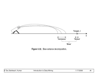
The Bias-Variance Decomposition (1) • Recall the expected squared loss, Lets denote, for simplicity: • Wesaidthatthesecond term corresponds to the noise inherent in the random variable t. • What about the first term?
The Bias-Variance Decomposition (2) Suppose we were given multiple data sets, each of size N. Any particular data set, D, will give a particular function y(x; D). Consider the error in the estimation:
The Bias-Variance Decomposition (3) Taking the expectation over D yields:
The Bias-Variance Decomposition (4) Thus we can write where
Bias measures how much the prediction (averaged over all data sets) differs from the desired regression function. • Variance measures how much the predictions for individual data sets vary around their average. • There is a trade-off between bias and variance • As we increase model complexity, • bias decreases (a better fit to data) and • variance increases (fit varies more with data)
f f bias gi g variance
Model Selection Procedures • Regularization (Breiman 1998): Penalize the augmented error: • error on data + l.model complexity • If l is too large, we risk introducing bias • Use cross validation to optimize for l • Structural Risk Minimization (Vapnik 1995): • Use a set of models ordered in terms of their complexities • Number of free parameters • VC dimension,… • Find the best model w.r.t empirical error and model complexity. • Minimum Description Length Principle • Bayesian Model Selection: If we have some prior knowledge about the approximating function, it can be incorporated into the Bayesian approach in the form of p(model).
Reminder: Introduction to OverfittingPRML 1.1 Concepts: Polynomial curve fitting, overfitting, regularization, training set size vs model complexity
Over-fitting Root-Mean-Square (RMS) Error:
Regularization One solution to control complexity is to penalize complex models -> regularization.
Regularization Use complex models, but penalize large coefficient values:
Regularization on 9th Order Polynomial ln l = -inf Too small l – no regularization effect
Regularization on 9th degree polynomial: Right l –good fit
Regularization: Large l –regularization dominates
The Bias-Variance Decomposition (5) Example: 100 data sets, each with 25 data points from the sinusoidal h(x) = sin(2px), varying the degree of regularization, l.
The Bias-Variance Decomposition (6) Regularization constant l = exp{-0.31}.
The Bias-Variance Decomposition (7) Regularization constant l = exp{-2.4}.
The Bias-Variance Trade-off From these plots, we note that; an over-regularized model (large l) will have a high bias while an under-regularized model (small l) will have a high variance. Minimum value of bias2+variance is around l=-0.31 This is close to the value that gives the minimum error on the test data.
f f bias gi g variance
Model Selection Procedures Cross validation: Measure the total error, rather than bias/variance, on a validation set. • Train/Validation sets • K-fold cross validation • Leave-One-Out • No prior assumption about the models