Download
1 / 166
1.66k likes | 1.78k Views
Scalable Performance Optimizations for Dynamic Applications. Laxmikant Kale http://charm.cs.uiuc.edu Parallel Programming Laboratory Dept. of Computer Science University of Illinois at Urbana Champaign. Scalability Challenges. Scalability Challenges Machines are getting bigger and faster

E N D
Scalable Performance Optimizations for Dynamic Applications Laxmikant Kale http://charm.cs.uiuc.edu Parallel Programming Laboratory Dept. of Computer Science University of Illinois at Urbana Champaign
Scalability Challenges • Scalability Challenges • Machines are getting bigger and faster • But • Communication Speeds? • Memory speeds? "Now, here, you see, it takes all the running you can do to keep in the same place" ---Red Queen to Alice in “Through The Looking Glass” • Further: • Applications are getting more ambitious and complex • Irregular structures and Dynamic behavior • Programming models?
Objectives for this Tutorial • Learn techniques that help achieve speedup • On Large parallel machines • On complex applications • Irregular as well as regular structures • Dynamic behaviors • Multiple modules • Emphasis on: • Systematic analysis • Set of techniques : a toolbox • Real life examples • Production codes (e.g. NAMD) • Existing machines
Current Scenario: Machines • Extremely High Performance machines abound • Clusters in every lab • GigaFLOPS per processor! • 100 GFLOPS/S performance possible • High End machines at centers and labs: • Many thousand processors, multi-TF performance • Earth Simulator, ASCI White, PSC Lemieux,.. • Future Machines • Blue Gene/L : 128k processors! • Blue Gene Cyclops Design: 1M processors • Multiple Processors per chip • Low Memory to Processor Ratio
Communication Architecture • On clusters: • 100 MB ethernet • 100 μs latency • Myrinet switches • User level memory-mapped communication • 5-15 μs latency, 200 MB/S Bandwidth.. • Relatively expensive, when compared with cheap PCs • VIA, Infiniband • On high end machines: • 5-10 μs latency, 300-500 MB/S BW • Custom switches (IBM, SGI, ..) • Quadrix • Overall: • Communication speeds have increased but not as much as processor speeds
Memory and Caches • Bottom line again: • Memories are faster, but not keeping pace with processors • Deep memory hierarchies: • On Chip and off chip. • Must be handled almost explicitly in programs to get good performance • A factor of 10 (or even 50) slowdown is possible with bad cache behavior • Increase reuse of data: If the data is in cache, use it for as many different things you need to do.. • Blocking helps
Application Complexity is increasing • Why? • With more FLOPS, need better algorithms.. • Not enough to just do more of the same.. • Better algorithms lead to complex structure • Example: Gravitational force calculation • Direct all-pairs: O(N2), but easy to parallelize • Barnes-Hut: N log(N) but more complex • Multiple modules, dual time-stepping • Adaptive and dynamic refinements • Ambitious projects • Projects with new objectives lead to dynamic behavior and multiple components
Disparity between peak and attained speed • As a combination of all of these factors: • The attained performance of most real applications is substantially lower than the peak performance of machines • Caution: Expecting to attain peak performance is a pitfall.. • We don’t use such a metric for our internal combustion engines, for example • But it gives us a metric to gauge how much improvement is possible
Overview • Programming Models Overview: • MPI • Virtualization and AMPI/Charm++ • Diagnostic tools and techniques • Analytical Techniques: • Isoefficiency, .. • Introduce recurring application Examples • Performance Issues • Define categories of performance problems • Optimization Techniques for each class • Case Studies woven through
Message Passing • Assume that processors have direct access to only their memory • Each processor typically executes the same executable, but may be running different part of the program at a time
Message passing basics: • Basic calls: send and recv • send(int proc, int tag, int size, char *buf); • recv(int proc, int tag, int size, char * buf); • Recv may return the actual number of bytes received in some systems • tag and proc may be wildcarded in a recv: • recv(ANY, ANY, 1000, &buf); • Global Operations: • broadcast • Reductions, barrier • Global communication: gather, scatter • MPI standard led to a portable implementation of these
MPI: Gather, Scatter, All_to_All • Gather (example): • MPI_Gather( sendarray, 100, MPI_INT, rbuf, 100, MPI_INT, root, comm); • Gets data collected at the (one) processor whose rank == root, of size 100*number_of_processors • Scatter • MPI_Scatter( sendbuf, 100, MPI_INT, rbuf, 100, MPI_INT, root, comm); • Root has the data, whose segments of size 100 are sent to each processor • Variants: • Gatherv, scatterv: variable amounts deposited by each proc • AllGather, AllScatter: • each processor is destination for the data, no root • All_to_all: • Like allGather, but data meant for each destination is different
Virtualization: Charm++ and AMPI • These systems seek an optimal division of labor between the “system” and programmer: • Decomposition done by programmer, • Everything else automated Decomposition Mapping Charm++ HPF Abstraction Scheduling Expression MPI Specialization
Virtualization: Object-based Decomposition • Idea: • Divide the computation into a large number of pieces • Independent of number of processors • Typically larger than number of processors • Let the system map objects to processors • Old idea? G. Fox Book (’86?), DRMS (IBM), .. • This is “virtualization++” • Language and runtime support for virtualization • Exploitation of virtualization to the hilt
Object-based Parallelization User is only concerned with interaction between objects System implementation User View
Data driven execution Scheduler Scheduler Message Q Message Q
Charm++ • Parallel C++ with Data Driven Objects • Object Arrays/ Object Collections • Object Groups: • Global object with a “representative” on each PE • Asynchronous method invocation • Prioritized scheduling • Mature, robust, portable • http://charm.cs.uiuc.edu
Charm++ : Object Arrays • A collection of data-driven objects (aka chares), • With a single global name for the collection, and • Each member addressed by an index • Mapping of element objects to processors handled by the system User’s view A[0] A[1] A[2] A[3] A[..]
Charm++ : Object Arrays • A collection of chares, • with a single global name for the collection, and • each member addressed by an index • Mapping of element objects to processors handled by the system User’s view A[0] A[1] A[2] A[3] A[..] System view A[0] A[3]
Chare Arrays • Elements are data-driven objects • Elements are indexed by a user-defined data type-- [sparse] 1D, 2D, 3D, tree, ... • Send messages to index, receive messages at element. Reductions and broadcasts across the array • Dynamic insertion, deletion, migration-- and everything still has to work!
Comparison with MPI • Advantage: Charm++ • Modules/Abstractions are centered on application data structures, • Not processors • Abstraction allows advanced features like load balancing • Advantage: MPI • Highly popular, widely available, industry standard • “Anthropomorphic” view of processor • Many developers find this intuitive • But mostly: • There is no hope of weaning people away from MPI • There is no need to choose between them!
Adaptive MPI • A migration path for legacy MPI codes • Allows them dynamic load balancing capabilities of Charm++ • AMPI = MPI + dynamic load balancing • Uses Charm++ object arrays and migratable threads • Minimal modifications to convert existing MPI programs • Automated via AMPizer • Bindings for • C, C++, and Fortran90
7 MPI processes AMPI:
7 MPI “processes” Real Processors AMPI: Implemented as virtual processors (user-level migratable threads)
Virtualization summary • Virtualization is • using many “virtual processors” on each real processor • A VP may be an object, an MPI thread, etc. • Charm++ and AMPI • Examples of programming systems based on virtualization • Virtualization leads to: • Message-driven (aka data-driven) execution • Allows the runtime system to remap virtual processors to new processors • Several performance benefits • For the purpose of this tutorial: • Just be aware that there may be multiple independent things on a PE • Also, we will use virtualization as a technique for solving some performance problems
Diagnostic tools • Categories • On-line, vs Post-mortem • Visualizations vs numbers • Raw data vs auto-analyses • Some simple tools (do it yourself analysis) • Fast (on chip) timers • Log them to buffers, print data at the end, • to avoid interference from observation • Histograms gathered at runtime • Minimizes amount of data to be stored • E.g. the number of bytes sent in each message • Classify them using a histogram array, • increment the count in one • Back of the envelope calculations!
Live Visualization • Favorite of CS researchers • What does it do: • As the program is running, you can see time varying plots of important metrics • E.g. Processor utilization graph, processor utilization shown as an animation • Communication patterns • Some researchers have even argued for (and developed) live sonification • Sound patterns indicate what is going on, and you can detect problems… • In my personal opinion, live analysis not as useful • Even if we can provide feedback to application to steer it, a program module can often do that more effectively (no manual labor!) • Sometimes it IS useful to have monitoring of application, but not necessarily for performance optimization
Postmortem data • Types of data and visualizations: • Time-lines • Example tools: upshot, projections, paragraph • Shows a line for each (selected) processor • With a rectangle for each type of activity • Lines/markers for system and/or user-defined events • Profiles • By modules/functions • By communication operations • E.g. how much time spent in reductions • Histograms • E.g.: classify all executions of a particular function based on how much time it took. • Outliers are often useful for analysis
Major analytical/theoretical techniques • Typically involves simple algebraic formulas, and ratios • Typical variables are: • data size (N), number of processors (P), machine constants • Model performance of individual operations, components, algorithms in terms of the above • Be careful to characterize variations across processors, and model them with (typically) max operators • E.g. max{Load I} • Remember that constants are important in practical parallel computing • Be wary of asymptotic analysis: use it, but carefully • Scalability analysis: • Isoefficiency
Scalability • The Program should scale up to use a large number of processors. • But what does that mean? • An individual simulation isn’t truly scalable • Better definition of scalability: • If I double the number of processors, I should be able to retain parallel efficiency by increasing the problem size
Equal efficiency curves Problem size processors Isoefficiency • Quantify scalability • How much increase in problem size is needed to retain the same efficiency on a larger machine? • Efficiency : Seq. Time/ (P · Parallel Time) • parallel time = computation + communication + idle • One way of analyzing scalability: • Isoefficiency: • Equation for equal-efficiency curves • Use η(p,N) = η(x.p, y.N) to get this equation • If no solution: the problem is not scalable • in the sense defined by isoefficiency
Introduction to recurring applications • We will use these applications for example throughout • Jacobi Relaxation • Classic finite-stencil-on-regular-grid code • Molecular Dynamics for biomolecules • Interacting 3D points with short- and long-range forces • Rocket Simulation • Multiple interacting physics modules • Cosmology / Tree-codes • Barnes-hut-like fast trees
Jacobi Relaxation Sequential pseudoCode: Decomposition by: While (maxError > Threshold) { Re-apply Boundary conditions maxError = 0; for i = 0 to N-1 { for j = 0 to N-1 { B[i,j] = 0.2(A[i,j] + A[I,j-1] +A[I,j+1] + A[I+1, j] + A[I-1,j]) ; if (|B[i,j]- A[i,j]| > maxError) maxError = |B[i,j]- A[i,j]| } } swap B and A } Row Blocks Or Column
Molecular Dynamics in NAMD • Collection of [charged] atoms, with bonds • Newtonian mechanics • Thousands of atoms (1,000 - 500,000) • 1 femtosecond time-step, millions needed! • At each time-step • Calculate forces on each atom • Bonds: • Non-bonded: electrostatic and van der Waal’s • Short-distance: every timestep • Long-distance: every 4 timesteps using PME (3D FFT) • Multiple Time Stepping • Calculate velocities and advance positions Collaboration with K. Schulten, R. Skeel, and coworkers
Traditional Approaches: non isoefficient • Replicated Data: • All atom coordinates stored on each processor • Communication/Computation ratio: P log P • Partition the Atoms array across processors • Nearby atoms may not be on the same processor • C/C ratio: O(P) • Distribute force matrix to processors • Matrix is sparse, non uniform, • C/C Ratio: sqrt(P) Not Scalable
Spatial Decomposition • Atoms distributed to cubes based on their location • Size of each cube : • Just a bit larger than cut-off radius • Communicate only with neighbors • Work: for each pair of nbr objects • C/C ratio: O(1) • However: • Load Imbalance • Limited Parallelism Cells, Cubes or“Patches”
Object Based Parallelization for MD: Force Decomposition + Spatial Deomp. • Now, we have many objects to load balance: • Each diamond can be assigned to any proc. • Number of diamonds (3D): • 14·Number of Patches
A C B Bond Forces • Multiple types of forces: • Bonds(2), Angles(3), Dihedrals (4), .. • Luckily, each involves atoms in neighboring patches only • Straightforward implementation: • Send message to all neighbors, • receive forces from them • 26*2 messages per patch! • Instead, we do: • Send to (7) upstream nbrs • Each force calculated at one patch
Virtualized Approach to implementation: using Charm++ 192 + 144 VPs 700 VPs 30,000 VPs These 30,000+ Virtual Processors (VPs) are mapped to real processors by charm runtime system
Rocket Simulation • Dynamic, coupled physics simulation in 3D • Finite-element solids on unstructured tet mesh • Finite-volume fluids on structured hex mesh • Coupling every timestep via a least-squares data transfer • Challenges: • Multiple modules • Dynamic behavior: burning surface, mesh adaptation Robert Fielder, Center for Simulation of Advanced Rockets Collaboration with M. Heath, P. Geubelle, others
Computational Cosmology • Here, we focus on n-body aspects of it • N particles (1 to 100 million), in a periodic box • Move under gravitation • Organized in a tree (oct, binary (k-d), ..) • Processors may request particles from specific nodes of the tree • Initialization and postmortem: • Particles are read (say in parallel) • Must distribute them to processor roughly equally • Must form the tree at runtime • Initially and after each step (or a few steps) • Issues: • Load balancing, fine-grained communication, tolerating communication latencies. • More complex versions may do multiple-time stepping Collaboration with T. Quinn, Y. Staedel, others
Causes of performance loss • If each processor is rated at k MFLOPS, and there are p processors, why don’t we see k•p MFLOPS performance? • Several causes, • Each must be understood separately, first • But they interact with each other in complex ways • Solution to one problem may create another • One problem may mask another, which manifests itself under other conditions (e.g. increased p).
Performance Issues • Algorithmic overhead • Speculative Loss • Sequential Performance • Critical Paths • Bottlenecks • Communication Performance • Overhead and grainsize • Too many messages • Global Synchronization • Load imbalance
Why Aren’t Applications Scalable? • Algorithmic overhead • Some things just take more effort to do in parallel • Example: Parallel Prefix (Scan) • Speculative Loss • Do A and B in parallel, but B is ultimately not needed • Load Imbalance • Makes all processor wait for the “slowest” one • Dynamic behavior • Communication overhead • Spending increasing proportion of time on communication • Critical Paths: • Dependencies between computations spread across processors • Bottlenecks: • One processor holds things up
Algorithmic Overhead • Sometimes, we have to use an algorithm with higher operation count in order to parallelize an algorithm • Either the best sequential algorithm doesn’t parallelize at all • Or, it doesn’t parallelize well (e.g. not scalable) • What to do? • Choose algorithmic variants that minimize overhead • Use two level algorithms • Examples: • Parallel Prefix (Scan) • Game Tree Search