Understanding Decision Trees in Computational Complexity<br>

1. P and NP

2. Computational Complexity • Recall from our sorting examples at the start of class that we could prove that any sort would have to do at least some minimal amount of work (lower bound) • We proved this using decision trees (ch 7.8) • (the following decision tree slides are repeated)

3. // Sorts an array of 3 items void sortthree(int s[]) { a=s[1]; b=s[2]; c=s[3]; if (a < b) { if (b < c) { S = a,b,c; } else { if (a < c) { S = a,c,b; } else { S = c,a,b; }} } else if (b < c) { if (a < c) { S = b,a,c; } else { S = b,c,a; }} else { S = c,b,a; } } a < b Yes No b < c b < c Yes No No Yes a,b,c a < c a < c c,b,a Yes No Yes No a,c,b c,a,b b,a,c b,c,a

4. Decision Trees • A decision tree can be created for every comparison-based sorting algorithm • The following is a decision tree for a 3 element Exchange sort • Note that “c < b” means that the Exchange sort compares the array item whose current value is c with the one whose current value is b – not that it compares s[3] to s[2].

5. b < a Yes No c < a c < b No Yes No Yes b < a c < a a < b c < b No Yes Yes Yes Yes No c,b,a b,c,a b,a,c c,a,b a,c,b a,b,c

6. Decision Trees • So what does this tell us… • Note that there are 6 leaves in each of the examples given (each N=3) • In general there will be N! leaves in a decision tree corresponding to the N! permutations of the array • The number of comparisons (“work”) is equal to the depth of the tree (from root to leaf) • Worst case behavior is the path from the root to the deepest leaf

7. Decision Trees • Thus, to get a lower bound on the worst case behavior we need to find the shortest tree possible that can still hold N! leaves • No comparison-based sort could do better • A tree of depth d can hold 2d leaves • So, what is the minimal d where 2d >= N! • Solving for d we get d >= log2(N!) • The minimal depth must be at least log2(N!)

8. Decision Trees • According to Lemma 7.4 (p. 291): log2(N!) >= n log2(n) – 1.45n • Putting that together with the previous result d must be at least as great as (n log2(n) – 1.45n) • Applying Big-O d must be at least O(n log2(n)) • No comparison-based sorting algorithm can have a running time better than O(n log2(n))

9. Decision Trees for other problems? • Unfortunately, this is a lot of work and the technique only applies directly to comparison-based sorts • What if the problem is Traveling Salesperson? • The book has only shown exponential time (or worse) algorithms for this problem • What if your boss wants a faster implementation? • Do you try and find one? • Do you try and prove one doesn’t exist?

10. Polynomial-Time Algorithms • A polynomial-time algorithm is one whose worst-case running time is bounded above by a polynomial function • Poly-time examples: 2n, 3n, n5, n log(n), n100000 • Non-poly-time examples: 2n, 20.000001n, n! • Poly-time is important because for large problem sizes, all non-poly-time algorithms will take forever to execute

11. Intractability • In Computer Science, a problem is called intractable if it is impossible to solve it with a polynomial-time algorithm • Let me stress that intractability is a property of the problem, not just of any one algorithm to solve the problem • There can be no poly-time algorithm that solves the problem if the problem is to be considered intractable • And just because one non-poly-time algorithm exists for the problem does not make it intractable

12. Three Categories of Problems • We can group problems into 3 categories: • Problems for which poly-time algorithms have been found • Problems that have been proven to be intractable • Proven that no poly-time algorithms exist • Problems that have not been proven to be intractable, but for which poly-time algorithms have never been found • No one has found a poly-time algorithm, but no one has proven that one doesn’t exist either • The interesting thing is that tons of problems fall into the 3rd category and almost none into the second

13. Poly-time Category • Any problem for which we have found a poly-time algorithm • Sorting, searching, matrix multiplication, chained matrix multiplication, shortest paths, minimal spanning tree, etc.

14. Intractable Category • Two types of problems • Those that require a non-polynomial amount of output • Determining all Hamiltonian Circuits • (n – 1)! Circuits in worst case • Those that produce a reasonable amount of output, but the processing time is just too long • These are called undecidable problems • Very few of these, but one classic is the Halting Problem • Takes as input any algorithm and any input and will tell you if the algorithm halts when run on the input

15. Unknown Category • Many problems belong in the category • 0-1 Knapsack, Traveling Salesperson, m-coloring, Hamiltonian Circuits, etc. • In general, any problem that we had to solve using backtracking or bounded backtracking falls into this category

16. The Theory of NP • In the following slides we will show a close and interesting relationship among many of the problem in the Unknown Category • It will be more convenient to develop this theory restricting ourselves to decision problems • Problems that have a yes/no answer • We can always convert non-decision problems into decision problems • In 0/1 Knapsack instead of just asking for the optimal profit, we can instead ask if the optimal profit exceeds some number • In graph coloring instead of just asking the minimal number of colors we can instead ask if the minimal number is less than m

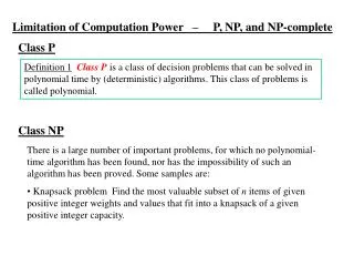
17. The Set P • The set P is the set of all decision problems that can be solved by polynomial-time algorithms • What problems are in P? • Obviously all the ones we have found poly-time solutions for (sorting, etc) • What about problems like Traveling Salesperson?

18. The Set NP • The set NP is the set of all decision problems that can be solved by a polynomial-time non-deterministic algorithm • A poly-time non-deterministic algorithm is an algorithm that is broken into 2 stages: • Guessing (non-deterministic) stage • Verification (deterministic) stage • Where the verification stage can be accomplished in poly-time

19. Non-deterministic Algorithms • For Traveling Salesperson: • The guessing stage simply guesses possible tours • The verification stage takes a tour from the guessing stage and decides yes/no • is it a tour that has a total weight of no greater than x? • Obviously, this verification stage can be written in poly-time • Note, however, that the guessing stage may or may not be done in poly-time • Note that the purpose of this type of algorithm is for theory and classification – there are usually much better ways to actually implement the algorithm

20. NP • There are thousands of problems that have been proven to be in NP • Further note that all problems in P are also in NP • The guessing stage can do anything it wants • The verification stage can just run the algorithm • The only problems proven to not be in NP are the intractable ones • And there are only a few of these

21. P and NP • Here is the way the picture of the sets is usually drawn • That is, we know that P is a subset of NP • However, we don’t know if it is a proper subset NP P

22. P and NP • That is, no one has ever proven that there exists a problem in NP that is not in P • So, NP – P could be an empty set • If it is then we say that P = NP • The question of whether P = NP is one of the more intriguing and important questions in all of Computer Science

23. P = NP? • To prove that P  NP we would have to find a single problem in NP that is not in P • To prove P = NP we would have to find a poly-time algorithm for each problem in NP • This route sounds much harder, but over the next few slides we will show a way to simplify this proof • If you prove either you get an A in the class, not to mention famous • And if you prove P = NP then you also become rich!

24. NP-Complete Problems • Over the next few slides we develop the background for a new set called NP-Complete • This set will help us in attempting to prove that P = NP

25. Conjunctive Normal Form (CNF) • A logical (boolean) variable is one that can have 2 values: true or false • A literal is a logical variable (x) or the negation of a logical variable (!x) • A clause is a sequence of literals separated by Ors: (x1 or x2 or !x3) • A logical expression in conjunctive normal form (CNF) is a sequence of clauses separated by ANDs: (x1 or x2 or !x3) and (x2 or !x1) and (x2 or x3) • We are about to use CNF for our theory, but there are many uses for CNF including AI

26. CNF-Satisfiability Problem • Given a logical expression in CNF, determine whether there is some truth assignment (some set of assignments of true and false to the variables) that makes the whole expression true • (x1 or x2) and (x2 or !x3) and (!x2) • Yes, x1 = true, x2 = false, x3 = false • (x1 or X2) and !x1 and !x2 • No

27. CNF-Satisfiability Problem • It is easy to write a poly-time algorithm that takes as input a logical expression in CNF and a set of true assignments a verifies if the expression is true for that assignment • Therefore, the problem is in the set NP • Further, no one has ever found a poly-time algorithm for this entire problem and no one has ever proven that it cannot be solved in poly-time • So we do not know if it is in P or not

28. CNF-Satisfiability Problem • However, in 1971 Stephen Cook published a paper proving that if CNF-Satisfiability is in P, then P = NP • WOW! If we can just prove that this simple problem is in P then suddenly all NP problems are in P • And all sorts of things like encryption will break! • Before we talk about how this works, we need to introduce the concept of a transformation algorithm

29. Transformation Algorithms • Suppose we want to solve decision problem A and we have an algorithm that solves decision problem B • Suppose that we can write an algorithm that creates an instance y of problem B for every instance x of problem A s.t. • The algorithm for B answers yes for y iff the answer to problem A is yes for x • Such an algorithm is called a transformation algorithm

30. Transformation Algorithms • An simple example of a transformation algorithm (having nothing to do with NP problems) • A: given n logical variables, does at least one have a value true? • B: Given n integers, is the largest of positive? • Our transformation is k1,k2..kn = tran(x1,x2..xn) • Where ki is 1 if xi is true and ki is 0 if xi is false

31. Reducibility • If there exists a poly-time transformation algorithm from decision problem A to decision problem B, then we say A is poly-time reducible to B (or A reduces to B) A  B • Further, if B is in set P and A  B then A is also in set P

32. NP-Complete Problems • A problem B is called NP-Complete if • It is in NP and • For every other problem A in NP, A  B • By the previous theorem if we could show that any NP-complete problem is in P then we could conclude that P = NP • So, Cook basically proved that CNF-Satisfiability is NP-complete • Cook did not reduce all other NP problems to CNF-Satisfiability, instead he did it by exploiting common properties of all NP problems

33. NP-Complete Problems • Now we can use transitivity to get: • A problem C is NP-complete if: • It is in NP and • For some other NP-complete problem B, B  C • Researchers have spent the last 30 years creating transformation for these problems and we now have a list of hundreds of NP-complete problems • If any of these NP-complete problems can be proven to be in P then P = NP • And, additionally, we also have a way to solve all the NP problems (poly-time transformations to the poly-time problem)

34. The State of P and NP • All this sounds promising, but… • Over the last 30 years no one has been able prove that any problem from NP is not in P • Over the last 30 years no one has been able to prove that any problem from NP-complete is in P • Proving either of these things would give us an answer to the open problem of P = NP? • Most people seem to believe that P  NP