Download
1 / 28
280 likes | 486 Views
Mesh-Based Inverse Kinematics. Robert W. Sumner Matthias Zwicker. Jovan Popovic MIT Craig Gotsman Harvard University. Demo. Demo. f 1. f 2. f 4. f 3. Compute Feature Vectors. f 5. w 2. w 3. w 4. w 5. w 1. Nonlinear Combination F= Σw i f i. w 6. w 10. f 6. w 7. w 9.

E N D
Mesh-Based Inverse Kinematics Robert W. Sumner Matthias Zwicker. Jovan Popovic MIT Craig Gotsman Harvard University
f1 f2 f4 f3 Compute Feature Vectors f5 w2 w3 w4 w5 w1 Nonlinear Combination F= Σwifi w6 w10 f6 w7 w9 w8 f7 f8 f9 f10
What is this paper about? • New framework – Feature Vectors • Traditional Point-based • Nonlinear mesh interpolation • Linear is good? • Efficient Optimization
Feature Vectors • Feature Vector = a group of deformation gradients. • What is deformation gradient • affine mapping is • Φ(p) = T*p + d, T = rotation, scaling, skewing • dΦ(p) / dp = T is deformation gradient • So given two triangles, how to find T? ┌ │ │ └ ┐ │ │ ┘ ┌ │ │ └ ┐ │ │ ┘ ┌ │ │ └ ┐ │ │ ┘ X Y Z d T X +
Deformed Reference
Feature Vectors • Deformation gradient of affine mapping • Φ(p) = T*p+d, T = rotation, scaling, skewing • Illustration in 2-D curve Φ1 Φ2 Φ3 Φ4 Φ5 Φ6 F = [T1, T2, T3, T4, T5, T6 ]T
In Mesh IK • Yet • Interpolation among feature vectors T1 T2 T3 T4 T5 T6 T d
Output Output Output Output ? In 3D ? Target
Output Output How it works? • Actually solving for position directly • x = argminx || f(x) - F || • f(x) = deformation gradient using x • x = argminx ||G’x – (F + c)||
Outline • New framework • Non-linear mesh interpolation • How to interpolate linearly? • Polar decomposition • Exponential map • Efficient Optimization
Linear Feature Space • We can find the desired mesh with feature vector fw = M*w, M is [f1,f2, … fn] • x*, w* = argmin || Gx – (Mw + c) || • If set Mw = davg + Σwidi • x*, w* = argmin || Gx – (Mw + c) || + k*||w|| ┌ │ │ │ │ └ ┐ │ │ │ │ ┘ *[1/3 2/3]T =
Alternative: Nonlinear • Polar decomposition • rotation & scaling differently • Exponential map • different interpolation • “Matrix animation and Polar Decomposition” - Shoemake & Duff • “Linear Combination of Transformation” - Marc Alexa
Polar Decomposition ┌ │ │ │ │ │ │ │ │ └ ┐ │ │ │ │ │ │ │ │ ┘ ┌ │ │ │ │ │ │ │ │ └ ┐ │ │ │ │ │ │ │ │ ┘ T1 T2 T3 . . . Tn R1S1 R2S2 R3S3 . . . RnSn = = R RS R must be orthogonal => SVD : UΣVT, QR : RL
Exponential Map For T x M = Tb x Ta x M if a = b = 1/2 So ½ T x ½ T = T => ½ of T = T ½ AxB = BxA? (Commutative) T = => Half T = => For T ½ ⊙ T ½ ⊙= exp( Log(A) + Log(B) ) T ½⊙ T ½= exp( ½ Log(T) + ½ Log(T) ) = T
Nonlinear Feature Space • Polar decomposition Tj = Rj * Sj, • Exponential map • Tj(w) = exp(Σwi*log(Rij)) * Σwi*Sij • We can find the desired mesh with feature vector fw = M*w = [f1,f2, … fn] * [w1, w2, … wn]T • Defined as fw = [T1(w1), T2(w2), … Tn(Wn)] = M(w) ┌ │ │ │ │ └ ┐ │ │ │ │ ┘ *[1/3 2/3]T =
Why use exponential map? • Easier to find derivatives, with respect to w • Tj(w) = R(w) * S(w) • dwkTj(w) = dR(w) * S(w) + R(w) * dS(w) • Then why do we need derivatives? • x*, w* = argmin || Gx – [M(w)+c] || • Gauss-Newton Algorithm • M(w +δ) = M(w) + dwM(w)* δ
Gauss-Newton Method • For k-th iteration: • δk, xk+1 = argmin||Gx – dwM(wk)*δ–(M(wk)+c)|| • wk+1 = wk + δk • ATA * [x, δ]T = AT( M(wk) + c ) • A = • Take about a minute or longer to solve ┌ │ │ └ ┐ │ │ ┘ G | - J1 G | - J2 G | - J3 Ji = dwM(w)
Outline • New framework • Non-linear mesh interpolation • Efficient Optimization • Specialized Cholesky-Factorization
Optimized Solver ATA * [x, δ]T = AT( M(wk) + c ) • General Cholesky or QR factorization might not suffice • The structure of ATA in previous normal equation is well defined ┌ │ │ └ ┐ │ │ ┘ G | - J1 G | - J2 G | - J3 A = ┌ │ │ │ └ ┐ │ │ │ ┘ GTG - GTJ1 GTG - GTJ2 GTG - GTJ3 - J1TG - J2TG - J3TG ΣJiTJi ATA =
Precomputation ATA * [x, δ]T = AT( M(wk) + c ) ┌ │ │ │ └ ┐ │ │ │ ┘ GTG - GTJ1 GTG - GTJ2 GTG - GTJ3 - J1TG - J2TG - J3TG ΣJiTJi ATA = Make U such that UTU = ATA ┌ │ │ │ └ ┐ │ │ │ ┘ ┌ │ │ └ ┐ │ │ ┘ R - R1 R - R2 R - R3 Rs G | - J1 G | - J2 G | - J3 U = A = where RTR = GTG, this R can be pre-computed
Solving for ┌ │ │ │ └ ┐ │ │ │ ┘ GTG - GTJ1 GTG - GTJ2 GTG - GTJ3 - J1TG - J2TG - J3TG ΣJiTJi = ATA = ┌ │ │ │ └ ┐ │ │ │ ┘ RTR - RTR1 RTR - RTR2 RTR - RTR3 - R1TR - R2TR - R3TR ΣRiTRi + RsTRs UTU = 1. Solve Ri ,where RTRi = GTJi, 1<=i<=3 2. Solve Rs ,where RsTRs = ΣJiTJi - RiTRi 3. The bottleneck for MeshIK