Download
1 / 30
300 likes | 466 Views
NAME Radar Data - Product Description & Quality Control. Guasave. Cabo. S-Pol. NAME Radar Network. Planned S-Pol 4 SMN Radars SMN radars run in full-volume 360s 15-min resolution Actual S-Pol (7/8-8/21) Cabo (7/15-Fall) Guasave (6/10-Fall)

E N D
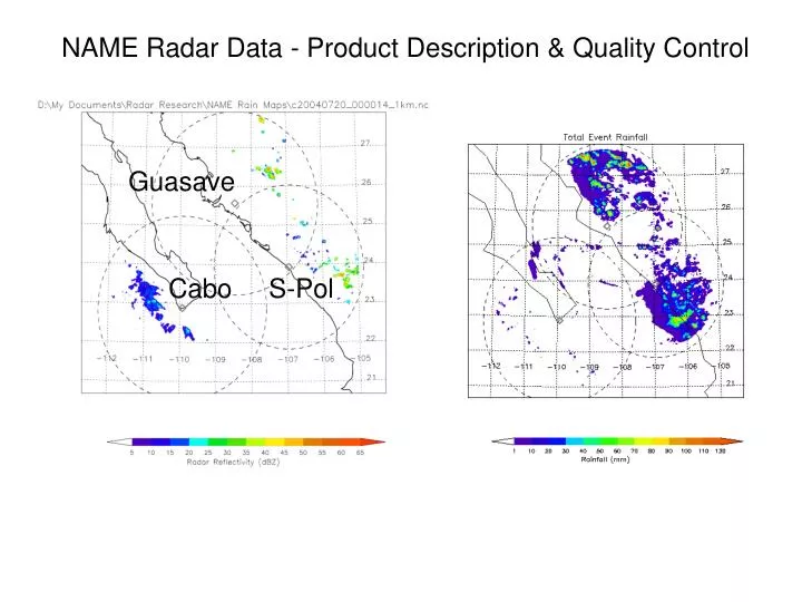
NAME Radar Data - Product Description & Quality Control Guasave Cabo S-Pol
NAME Radar Network Planned • S-Pol • 4 SMN Radars • SMN radars run in full-volume 360s • 15-min resolution Actual • S-Pol (7/8-8/21) • Cabo (7/15-Fall) • Guasave (6/10-Fall) • SMN radars single low-level sweep (high temporal resolution)
S-Pol Operations 24-h Ops started 7/8, continued through 8/21 Occasional downtime for Ka-band work in preparation for RICO – Usually mid-morning precipitation minimum Two Modes of Scanning: “Climatology” Used most frequently 200-km range Full-volume 360s, completed in 15-min Includes rain-mapping angles (0.8,1.3,1.8-deg) & 0.0-deg “Storm Microphysics” 70-80 hours total spread over ~35 cases Usually 150-km range 2-3 sector PPI volumes with 0-1 sets of RHIs in 15 min Includes 360s @ rain-mapping angles (0.8,1.3,1.8-deg)
Insect Filtering Thresholds found empirically More stringent than TRMM-LBA Courtesy of Lee Nelson
Other Thresholds Standard Deviation of Differential Phase (Z-dependent) [Std Dev of Phase determined over 11 gates; used to be 21] Correlation Coefficient (range-dependent) LDR & Differential Phase (Second Trip) Test pulse removed via range filter, sometimes hand edit [Did not check all sweeps, only 0.8, 1.3, 1.8 SUR]
S-Pol Differential Phase Filtering and KDP Calculation Differential phase was filtered using a 21-gate (3.15-km) finite impulse response filter developed by John Hubbert of NCAR and V. N. Bringi of Colorado State University. Small data gaps (less than 20%; used to be 50%) within this moving window were filled using linear interpolation, in order to increase the amount of usuable windows for subsequent specific differential phase (KDP) calculation. KDP was calculated from the slope of a line fitted to the filtered differential phase field. The window over which this line was fitted changed depending on the Z of the central gate. If Z < 35 dBZ, then we fitted to 31 gates (4.65 km). For Z between 35 and 45 dBZ, we fitted to 21 gates (3.15 km). For Z > 45 dBZ, we fitted to 11 gates (1.65 km). This allowed for more accurate KDP estimates at both high and low Z. For a handful of sweeps during a major storm on 8/3, we found that differential phase became folded due to the large areas of intense rain. Prior to filtering and KDP estimation, we unfolded the differential phase field by hand using soloii.
Gaseous Attenuation Correction Battan (1973)
Polarimetric Correction of Rain Attenuation Find Slope of Line This is Decrease in Z per Degree of Phase Shift Do Same Thing for ZDR
Fuzzy-Logic Based Hydrometeor ID Lt Green - Snow, Dk Green - Rain, Yellows - Graupel Follow Tessendorf et al. (2005) using mean sounding No Mixed Precip Categories Run ID in polar coordinates
S-Pol Compositing - Old Methodology Only correct up to 5 dBZ before moving to next angle
Mean Reflectivity (Avg’d in Log Space) Old Methodology, Entire Project
Low Bias At Long Range Behind Block
Changes to Blockage Correction Much more stringent KDP calculation Requirements on KDPand HID (formerly just KDP) Using entire dataset (formerly just 1 week) Added Giangrande et al. (2005) correction for ZDR (formerly set to missing in blocks)
ZDR in Light Rain, Entire Project Giangrande et al. (2005) Methodology
S-Pol Corrected Sweeps 0.5, 0.8, 1.0, 1.3, 1.4, 1.5, 1.8, 2.0 (PPIs and SURs) (0.8, 1.3, 1.8 have best confidence for Z) Not Corrected 0.0, 0.2, 0.3, 0.4, 0.6, 0.7, 0.9, 1.2, 1.6, 1.7, 1.9 All RHIs Not Requiring Correction 2.1+
S-Pol Intercomparison with TRMM 8/18 0304 UTC
S-Pol Intercomparison with TRMM 8/10 0045 UTC
SMN QC 1. Sorted Into 15-Minute Periods 2. Threshold on Z, NCP, Power - Then Despeckle 3. Correct Guasave Azimuths Due To Backlash 4. Clutter Filter For Guasave Developed Using Clear-Air 5. Hand Edit Remaining Spurious Echo Using soloii 6. Calibrated Via Intercomparison with S-Pol 7. Correct Attenuation Using GATE Algorithm (Z=221R1.25) Final Sensitivity: 10-20 dBZ Minimum Detectable
New Product Courtesy of Steve Nesbitt IR Brightness Temperature On Same Grid As Radar Data 2 & 5 km Resolutions Available
Sea Clutter Near Cabo Easily Identified, If We Had Higher Angle Sweeps!
Density of Points, TB vs. Z Sea Clutter Entire Project, All Points Where Z & TB Are Not Missing
Density of Points, TB vs. Z Sea Clutter Cabo Area (West of 109W, South of 25N) Suggested Filter: Ignore Z w/ TB 290K
TO DO LIST 1. Double-Check Z-R Via Intercomparison With Gages 2. Check Capping of Z-R (Ice Contamination) 3. Create S-Pol Rain Map Composites Using Higher Angles (4. Quantify rainfall errors) Then Send Data to NCAR to Create v2 Regional Composites 3-D S-Pol Data Ready for Research Now! (PPIs, SURs, RHIs; watch out for test pulse) v1 composites in /net/andes/data2/tlang/name
Guasave /net/andes/data2/tlang/smn/guasave/qc (DZA & RR) Cabo /net/andes/data2/tlang/smn/cabo/qc (DZA & RR) S-Pol /net/cook/data/name/spol/NAME_sweeps (thru 8/17) /net/shasta/data/tlang/name (8/18-8/21) (DZC & DRC) USE NCSWP FILES!!!!!!!!!!!!!!!!!!!!!!!!!!!!!!!!!!!!!!!!!!!!!!!
Version 3? Use FHC-based data filtering