Download
1 / 20
220 likes | 474 Views
Spherical Harmonic Lighting: The Gritty Details(1/3). Shader Study 임정환 발표 08/04/15. 발표를 하게된 이유. ShaderX4 2.9 Dynamical global illuminations using Tetrahedron environment mapping 모름 PRT -> 모름 BRDF -> 모름 안에 사용된 SH -> 모름 OTL 걍 처음부터 …. Introduction.

E N D
Spherical Harmonic Lighting:The Gritty Details(1/3) Shader Study 임정환 발표 08/04/15
발표를 하게된 이유 • ShaderX4 2.9 Dynamical global illuminations using Tetrahedron environment mapping모름 • PRT -> 모름 • BRDF -> 모름 • 안에 사용된 SH -> 모름 • OTL • 걍 처음부터…
Introduction • Precomputed Radiance Transfer for Real-Time Rendering. in Dynamic, Slon(02) • Realtime Global Illumination의 한 획을 그은 역사적인 논문 • 문제는? • 어렵다. • 복잡하다. • 넘 많은 기초지식을 요해.. • OTL • 해서 우리의 Robin Green께서 Spherical Harmonic Lighting:The Gritty Details 이라는 논문을 내셨다!! • 해도 넘 어렵더라 • 공업수학 내용 나오고, 돌아버림
Introduction • 발표순서는 • 1페이지부터 순서대로.. • 모두 이해되면 다시한번(No 순서대로)
Illumination Calculations(2~3쪽) • Diffuse Surface Reflection • The Rendering Equation, differential angle form
Illumination Calculations(4쪽) • 용어들 • Flux = joules/second (watt) • 얼마나 많은 photon이 unit시간당 면에 부딪히는가? • 면이 넓으면 값이 커짐 • Irradiance(조사) = watt/meter2 • Projected Solid Angle 을 통해 들어오는 빛들을 구면전체로 적분을 하면 빛의 밝기가 결정된다… • 어떻게 위의 수식들을 리얼타임으로 표현할 것인가?
Monte Carlo Integration(4쪽) • 어떻게 적분할 것인가? • 몬테카를로!! • 몬테카를로는 Probability(확률)에 기반한 방법 • f(x)는 일반적인 함수 • P(x)는 cummulative distribution function(축적된 배분함수) • F(x)의 각 부분에 대해서 얼마나 자주 불릴 것인가에 대한 확률을 나타내는 확률함수 • 예제: 주사위(1~6)를 굴렸을때 4이하일 P(4)는 2/3 • 만약 모든 범위에서 확률이 같다면 uniform random variable이라 한다.
Monte Carlo Integration(5쪽) • Probability density function • p(x) • x가 a와 b사이의 값일 확률 • 평균값(기대값) • 예제 f(x)=2-x 라는 함수에서 0~2사이의 값의 기대값(평균)을 구하라.. • 확률이 uniform random variable 이므로 p(x)=1/2
Monte Carlo Integration(6쪽) • 위의 방법은 적분해서 기대값을 구하는 방법…허나 컴퓨터에서 하기에는 무리 • 또다른 방법은? • 열나게 샘플링해서 평균내기! • 이제 f(x)를 적분해 보자. • f(x)를 아주 많이 sample하의 값을 얻고 • PDF값( p(x) )로 scaling 한후 • 결과값들을 합한후에 • sample수로 나누면 f(x)의 적분값을 구할 수 있다. • sampling을 많이 할수록 정확한 값을 구할 수 있다 • p(x)=f(x)다면 한번만 샘플링해도 된다.
Monte Carlo Integration(6쪽) • 위의 식의 또다른 표현법은 • 자.. 그러면 우리가 할일 • p(x)를 uniform하게 분포시켜주면 최대한 적게 샘플링하더라도 f(x)의 적분값을 approximate 할 수 있는 것이다. • 구의 표면에서 우리는 적분을 할 것이므로 최대한 고르게 sample을 분산시켜주는 것이 목표 • 이것을 unbiased random samples이라 한다. • 구에서는 한쌍의 independent canonical random number ξx 와 ξy 값을 구한후 값을 바꾸어 구상에서 맵핑값으로 사용할 수 있다. Mapping [0..1,0..1] random numbers into spherical coordinates.
Monte Carlo Integration(7쪽) • 자.. 좀 더샘플링값을 낮추어 보자 • jittered sample • stratified sampling(층을 나누는 샘플링) • N*N의 cell로 나누고 • 각 cell마다 random point를 뽑자. • 각셀의 편차의 합은 전체 범위에서 샘플했을때보다 크지않더라.. 즉 고르게 되더라..
Monte Carlo Integration(7쪽) • 지금까지 결과를 코드로 정리해보자. void SH_setup_spherical_samples(SHSample samples[], int sqrt_n_samples) { // fill an N*N*2 array with uniformly distributed // samples across the sphere using jittered stratification int i=0; // array index double oneoverN = 1.0/sqrt_n_samples; for(int a=0; a<sqrt_n_samples; a++) { for(int b=0; b<sqrt_n_samples; b++) { // generate unbiased distribution of spherical coords double x = (a + random()) * oneoverN; // do not reuse results double y = (b + random()) * oneoverN; // each sample must be random double theta = 2.0 * acos(sqrt(1.0 - x)); double phi = 2.0 * PI * y; samples[i].sph = Vector3d(theta,phi,1.0); // convert spherical coords to unit vector Vector3d vec(sin(theta)*cos(phi), sin(theta)*sin(phi), cos(theta)); samples[i].vec = vec; // precompute all SH coefficients for this sample for(int l=0; l<n_bands; ++l) { for(int m=-l; m<=l; ++m) { int index = l*(l+1)+m; samples[i].coeff[index] = SH(l,m,theta,phi); } } ++i; } } } struct SHSample { Vector3d sph; Vector3d vec; double *coeff; };
Orthogonal Basis Function(8쪽) • Basis function( Bi(x) ) • 어떤 original function을 나타낼수있는 작은 조각 • basis function을 scaling, sum을 통해 original function을 근사화할 수 있다.(이러한 과정을 projection한다고 한다) 옆에 과정을 통해 coefficient를 구할 수 있다. 구해진 coefficient와 basis를 한번 더 곱한 후 그 결과값을 sum하자
Orthogonal Basis Function(9쪽) • 방금전에 사용된 것은 linear basis functions으로 input function으로 piecewise linear approximation(구분적 선형 근사)을 준다. • 여러 basis function이 있지만 orthogonal polynomials라 불리는 것이 많이 사용됨 • Orthogonal polynomials(직교 다항식) • 성질 • 직관적으로 다항식들간의 간섭하지 않는다는 것을 알 수 있다. • 가장 유명한 것 중 Legendre polynomials 라 불리는 것이 있다. • Associated Legendre polynomials • symbol로 P라고 표현 • l과 m으로 표현 (-1~1사이) • real number(실수)를 반환
Orthogonal Basis Function(9쪽) • Associated Legendre polynomials • 2개의 아규먼트 l,m은 polynomial을 여러 개의 function band로 나눈다. • l은 band index , 0을 포함한 양수 • m은 0~l사이의 값 The first six associated Legendre polynomials. 위와 같이 n개면 n(n+1)개의 coefficient를 구한다.
Orthogonal Basis Function(10쪽) • Associated Legendre polynomials • 각각의 polynomial을 recursive하게 나타낼수있다. • 아래 세가지 법칙에 따라..
Orthogonal Basis Function(10~11쪽) • Associated Legendre polynomials • 소스코드로 한 번 살펴보자
Spherical Harmonics(11~12쪽) • SH함수는 일반적으로 복소수에서 정의가 되나, 여기서는 근사화된 실수 범위에서 정의 l과 m은 좀 Legendre polynomial과는 좀 다른데 –l이 0을포함한 양수 m은 –ㅣ ~ ㅣ사이의 값
Spherical Harmonics(13쪽) • 소스코드를 보자