Download
1 / 30
310 likes | 552 Views
Fourier vs Wavelets. Researchlab 4 Presentation. Maurice Samulski June 27 th , 2005. Contents. Introduction Discrete Fourier Transform Discrete Cosine Transform Wavelet Transform Comparison between DCT and WT Conclusions. Wednesday, June 4, 2014 Research Lab 4 presentation. 2.

E N D
Fourier vs Wavelets Researchlab 4 Presentation Maurice Samulski June 27th, 2005
Contents • Introduction • Discrete Fourier Transform • Discrete Cosine Transform • Wavelet Transform • Comparison between DCT and WT • Conclusions Wednesday, June 4, 2014 Research Lab 4 presentation 2
Fourier analysis • Joseph Fourier 1807 • Represent functions by superposing sines and cosines with different frequencies and amplitudes • s(t) = 3 sin (t) - 100 sin(4t) - 20 sin (200t) Wednesday, June 4, 2014 Research Lab 4 presentation 3
Fourier analysis Wednesday, June 4, 2014 Research Lab 4 presentation 4
Discrete Fourier Transform (DFT) • DFT of image f(x,y) with size m x n Wednesday, June 4, 2014 Research Lab 4 presentation 5
Discrete Fourier Transform (DFT) • Inverse DFT of F(u,v) Wednesday, June 4, 2014 Research Lab 4 presentation 6
Discrete Fourier Transform • Image f(x,y) is real • Fourier transform F(u,v) is complex • F(u,v) often represented as Wednesday, June 4, 2014 Research Lab 4 presentation 7
Discrete Fourier Transform Wednesday, June 4, 2014 Research Lab 4 presentation 8
Discrete Fourier Transform Wednesday, June 4, 2014 Research Lab 4 presentation 9
Discrete Fourier Transform Wednesday, June 4, 2014 Research Lab 4 presentation 10
Discrete Cosine Transform (DCT) • Very similar to the discrete Fourier transform, but • Uses only real numbers • Decomposes a function into a series of even cosine components only • Different ordering of coefficients • Computationally cheaper than DFT and therefore very commonly used in image processing, eg JPEG and MPEG Wednesday, June 4, 2014 Research Lab 4 presentation 11
(1) Divide image into 8x8 blocks 8x8 block Input image Wednesday, June 4, 2014 Research Lab 4 presentation 12
(2a) 2-D DCT basis functions Low High Low Low High High 8x8 block High Low Wednesday, June 4, 2014 Research Lab 4 presentation 13
(2b) 2-D Transform Coding DC coefficient (average color) + y00 y23 y12 y01 y10 ... AC coefficients (details) Wednesday, June 4, 2014 Research Lab 4 presentation 14
(3) Zig-zag ordering DCT blocks • Why? To group low frequency coefficients in top of vector. • Maps 8 x 8 to a 1 x 64 vector. Wednesday, June 4, 2014 Research Lab 4 presentation 15
DCT compression • Because human eye is most sensitive to low frequencies, less sensitive to high frequencies, we can truncate the coefficients which represent these high frequencies • The lower quality setting, the more coefficients are truncated • Lesser coefficients mean less detail of the block which leads to the famous blocking artifact Wednesday, June 4, 2014 Research Lab 4 presentation 16
Wavelets • The major advantage of using wavelets is that they can be used for analyzing functions at various scales • It stores versions of an image at various resolutions, which is very similar how the human eye works. • As you zoom in at smaller and smaller scales, you can find details that you did not see before. Wednesday, June 4, 2014 Research Lab 4 presentation 17
Haar wavelet example (1D) • Suppose we have a one-dimensional data set containing eight pixels: [ 10 8 6 8 1 5 8 2 ] • We can represent this image in the Haar basis by computing a wavelet transform, by averaging the pixels together pairwise: [ 9 7 3 5 ] • Clearly, some information has been lost in this averaging process, we need to store detail coefficients: [ 1 -1 -2 1 ] Wednesday, June 4, 2014 Research Lab 4 presentation 18
Haar wavelet example (1D) • The full decomposition will look like • We will store this as follows: [ 6 2 1 −1 1 −1 −2 1 ] • No information has been gained or lost by this process Wednesday, June 4, 2014 Research Lab 4 presentation 19
Haar wavelet example (1D) • The full decomposition will look like • This transform will be stored as: [ 6 2 1 −1 1 −1 −2 1 ] • No information has been gained or lost by this process Wednesday, June 4, 2014 Research Lab 4 presentation 20
Haar wavelet • This may look wonderful and all, but what good is compression that takes eight values and compresses it to eight values? • Pixel values are similar to their neighbors • The image can be compressed by removing small coefficients from this transform • The one-dimensional Haar Transform can be easily extended to two-dimensional • Input matrix instead of an input vector • apply the one-dimensional Haar transform on each row • apply the one-dimensional Haar transform on each column Wednesday, June 4, 2014 Research Lab 4 presentation 21
Other wavelets • The Haar wavelet uses simple basis functions (discontinuous) for scaling and determining detail coefficients • Not suitable for smooth functions Wednesday, June 4, 2014 Research Lab 4 presentation 22
JPEG vs JPEG2000 • Generally, there are two visible damages caused by image compression: • Blocking artifacts: artificial horizontal and vertical borders between blocks • Blur: loss of fine detail and the smearing of edges Wednesday, June 4, 2014 Research Lab 4 presentation 23
Test: Image quality • Test results are subjective • With ‘normal’ compression (2+ bits/pixel), quality advantage of JPEG2000 is negligible • Real quality advantage will only become clear by using very high compression ratios (0.5 or less b/p) • At 0.25 b/p, JPEG images begin to look like a mosaic while with JPEG2000 it gets a elegant blur across the image • JPEG2000 image files tend to be 20 to 60% smaller than their JPEG counterparts for the same subjective image quality Wednesday, June 4, 2014 Research Lab 4 presentation 24
Test: Image quality (Original) Lena Original (512x512x24b) Building Plan (small piece) Wednesday, June 4, 2014 Research Lab 4 presentation 25
Results: Image quality (Lena) JPEG (0.2 b/p) JPEG2000 (0.2 b/p) Wednesday, June 4, 2014 Research Lab 4 presentation 26
Results: Image quality (Building plan) JPEG (0.2 b/p) JPEG2000 (0.2 b/p) Wednesday, June 4, 2014 Research Lab 4 presentation 27
Results: Performance • Price to pay: considerable increase in computational complexity and memory usage Wednesday, June 4, 2014 Research Lab 4 presentation 28
Conclusions • JPEG2000 works better with sharp spikes in images • Quality advantages are really visible when compressing with very high compression ratios • Only to be used with very large datasets like fingerprints, MRI scans, building plans, etc. • You can choose between different wavelet basis functions to get the optimal result for a specific application • Blur isn’t experienced as bad as blocking artifacts • Time needed to compress high resolution images takes a lot of time with JPEG2000 Wednesday, June 4, 2014 Research Lab 4 presentation 29
Questions? Wednesday, June 4, 2014 Research Lab 4 presentation 30