Download
1 / 130
1.31k likes | 1.35k Views
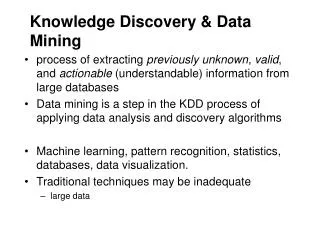
Explore the motivation, applications, and techniques behind data mining in various fields such as homeland security, business, scientific data, and health sciences. Learn about predictive modeling, classification tasks, and building classification models.

E N D
Knowledge Discovery and Data Mining from Big Data Vipin Kumar Department of Computer Science University of Minnesota kumar@cs.umn.eduwww.cs.umn.edu/~kumar
Mining Big Data: Motivation • Today’s digital society has seen enormous data growth in both commercial and scientific databases • Data Mining is becoming a commonly used tool to extract information from large and complex datasets • Examples: • Helps provide better customer service in business/commercial setting • Helps scientists in hypothesis formation Homeland Security Business Data Geo-spatial data Computational Simulations Sensor Networks Scientific Data
Data Mining for Life and Health Sciences • Recent technological advances are helping to generate large amounts of both medical and genomic data • High-throughput experiments/techniques • Gene and protein sequences • Gene-expression data • Biological networks and phylogenetic profiles • Electronic Medical Records • IBM-Mayo clinic partnership has created a DB of 5 million patients • Single Nucleotides Polymorphisms (SNPs) • Data mining offers potential solution for analysis of large-scale data • Automated analysis of patients history for customized treatment • Prediction of the functions of anonymous genes • Identification of putative binding sites in protein structures for drugs/chemicals discovery Protein Interaction Network
Origins of Data Mining • Draws ideas from machine learning/AI, pattern recognition, statistics, and database systems • Traditional Techniquesmay be unsuitable due to • Enormity of data • High dimensionality of data • Heterogeneous, distributed nature of data Statistics/AI Machine Learning/ Pattern Recognition Data Mining Database systems
Data Mining Tasks... Data Clustering Predictive Modeling Anomaly Detection Association Rules Milk
Test Set Model General Approach for Building a Classification Model quantitative categorical categorical class Learn Classifier Training Set
Examples of Classification Task • Predicting tumor cells as benign or malignant • Classifying secondary structures of protein as alpha-helix, beta-sheet, or random coil • Predicting functions of proteins • Classifying credit card transactions as legitimate or fraudulent • Categorizing news stories as finance, weather, entertainment, sports, etc • Identifying intruders in the cyberspace
Commonly Used Classification Models • Base Classifiers • Decision Tree based Methods • Rule-based Methods • Nearest-neighbor • Neural Networks • Naïve Bayes and Bayesian Belief Networks • Support Vector Machines • Ensemble Classifiers • Boosting, Bagging, Random Forests
Model for predicting credit worthiness Employed Yes No No Education { High school, Graduate Undergrad } Number of Yes years > 7 yrs < 7 yrs Yes No Classification Model: Decision Tree Class
Employed Yes Yes No No Education Worthy: 4 Not Worthy:3 Worthy: 4 Not Worthy:3 Worthy: 0 Not Worthy:3 Worthy: 0 Not Worthy:3 Graduate High School/ Undergrad Worthy: 2 Not Worthy:2 Worthy: 2 Not Worthy:4 Not Worthy Worthy 4 3 Employed = Yes Key Computation 0 3 Employed = No Constructing a Decision Tree Employed
Constructing a Decision Tree Employed = Yes Employed = No
Design Issues of Decision Tree Induction • How should training records be split? • Method for specifying test condition • depending on attribute types • Measure for evaluating the goodness of a test condition • How should the splitting procedure stop? • Stop splitting if all the records belong to the same class or have identical attribute values • Early termination
How to determine the Best Split • Greedy approach: • Nodes with purer class distribution are preferred • Need a measure of node impurity: High degree of impurity Low degree of impurity
Measure of Impurity: GINI • Gini Index for a given node t : (NOTE: p( j | t) is the relative frequency of class j at node t). • Maximum (1 - 1/nc) when records are equally distributed among all classes, implying least interesting information • Minimum (0.0) when all records belong to one class, implying most interesting information
Measure of Impurity: GINI • Gini Index for a given node t : (NOTE: p( j | t) is the relative frequency of class j at node t). • For 2-class problem (p, 1 – p): • GINI = 1 – p2 – (1 – p)2 = 2p (1-p)
Computing Gini Index of a Single Node P(C1) = 0/6 = 0 P(C2) = 6/6 = 1 Gini = 1 – P(C1)2 – P(C2)2 = 1 – 0 – 1 = 0 P(C1) = 1/6 P(C2) = 5/6 Gini = 1 – (1/6)2 – (5/6)2 = 0.278 P(C1) = 2/6 P(C2) = 4/6 Gini = 1 – (2/6)2 – (4/6)2 = 0.444
Computing Gini Index for a Collection of Nodes • When a node p is split into k partitions (children) where, ni = number of records at child i, n = number of records at parent node p. • Choose the attribute that minimizes weighted average Gini index of the children • Gini index is used in decision tree algorithms such as CART, SLIQ, SPRINT
Binary Attributes: Computing GINI Index • Splits into two partitions • Effect of Weighing partitions: • Larger and Purer Partitions are sought for. B? Yes No Node N1 Node N2 Gini(N1) = 1 – (5/6)2 – (1/6)2= 0.278 Gini(N2) = 1 – (2/6)2 – (4/6)2= 0.444 Weighted Gini of N1 N2= 6/12 * 0.278 + 6/12 * 0.444= 0.361 Gain = 0.486 – 0.361 = 0.125
Continuous Attributes: Computing Gini Index • Use Binary Decisions based on one value • Several Choices for the splitting value • Number of possible splitting values = Number of distinct values • Each splitting value has a count matrix associated with it • Class counts in each of the partitions, A < v and A v • Simple method to choose best v • For each v, scan the database to gather count matrix and compute its Gini index • Computationally Inefficient! Repetition of work.
Decision Tree Based Classification • Advantages: • Inexpensive to construct • Extremely fast at classifying unknown records • Easy to interpret for small-sized trees • Robust to noise (especially when methods to avoid overfitting are employed) • Can easily handle redundant or irrelevant attributes (unless the attributes are interacting) • Disadvantages: • Space of possible decision trees is exponentially large. Greedy approaches are often unable to find the best tree. • Does not take into account interactions between attributes • Each decision boundary involves only a single attribute
Handling interactions + : 1000 instances o : 1000 instances Entropy (X) : 0.99 Entropy (Y) : 0.99 Y X
Handling interactions + : 1000 instances o : 1000 instances Adding Z as a noisy attribute generated from a uniform distribution Entropy (X) : 0.99 Entropy (Y) : 0.99 Entropy (Z) : 0.98 Attribute Z will be chosen for splitting! Y X Z Z X Y
Limitations of single attribute-based decision boundaries Both positive (+) and negative (o) classes generated from skewed Gaussians with centers at (8,8) and (12,12) respectively.
Classification Errors • Training errors (apparent errors) • Errors committed on the training set • Test errors • Errors committed on the test set • Generalization errors • Expected error of a model over random selection of records from same distribution
Example Data Set Two class problem: + : 5200 instances • 5000 instances generated from a Gaussian centered at (10,10) • 200 noisy instances added o : 5200 instances • Generated from a uniform distribution 10 % of the data used for training and 90% of the data used for testing
Decision Tree with 4 nodes Decision Tree Decision boundaries on Training data
Decision Tree with 50 nodes Decision Tree Decision Tree Decision boundaries on Training data
Which tree is better? Decision Tree with 4 nodes Which tree is better ? Decision Tree with 50 nodes
Model Overfitting Underfitting: when model is too simple, both training and test errors are large Overfitting: when model is too complex, training error is small but test error is large
Model Overfitting Using twice the number of data instances • If training data is under-representative, testing errors increase and training errors decrease on increasing number of nodes • Increasing the size of training data reduces the difference between training and testing errors at a given number of nodes
Reasons for Model Overfitting • Presence of Noise • Lack of Representative Samples • Multiple Comparison Procedure
Effect of Multiple Comparison Procedure • Consider the task of predicting whether stock market will rise/fall in the next 10 trading days • Random guessing: P(correct) = 0.5 • Make 10 random guesses in a row:
Effect of Multiple Comparison Procedure • Approach: • Get 50 analysts • Each analyst makes 10 random guesses • Choose the analyst that makes the most number of correct predictions • Probability that at least one analyst makes at least 8 correct predictions
Effect of Multiple Comparison Procedure • Many algorithms employ the following greedy strategy: • Initial model: M • Alternative model: M’ = M , where is a component to be added to the model (e.g., a test condition of a decision tree) • Keep M’ if improvement, (M,M’) > • Often times, is chosen from a set of alternative components, = {1, 2, …, k} • If many alternatives are available, one may inadvertently add irrelevant components to the model, resulting in model overfitting
Effect of Multiple Comparison - Example Use additional 100 noisy variables generated from a uniform distribution along with X and Y as attributes. Use 30% of the data for training and 70% of the data for testing Using only X and Y as attributes
Notes on Overfitting • Overfitting results in decision trees that are more complex than necessary • Training error does not provide a good estimate of how well the tree will perform on previously unseen records • Need ways for incorporating model complexity into model development
Evaluating Performance of Classifier • Model Selection • Performed during model building • Purpose is to ensure that model is not overly complex (to avoid overfitting) • Model Evaluation • Performed after model has been constructed • Purpose is to estimate performance of classifier on previously unseen data (e.g., test set)
Methods for Classifier Evaluation • Holdout • Reserve k% for training and (100-k)% for testing • Random subsampling • Repeated holdout • Cross validation • Partition data into k disjoint subsets • k-fold: train on k-1 partitions, test on the remaining one • Leave-one-out: k=n • Bootstrap • Sampling with replacement • .632 bootstrap:
Application : SNP Association Study • Given: A patient data set that has genetic variations (SNPs) and their associated Phenotype (Disease). • Objective: Finding a combination of genetic characteristics that best defines the phenotype under study. Genetic Variation in Patients (SNPs) as Binary Matrix and Survival/Disease (Yes/No) as Class Label. Genetic Variation in Patients (SNPs) as Binary Matrix and Survival/Disease (Yes/No) as Class Label. Genetic Variation in Patients (SNPs) as Binary Matrix and Survival/Disease (Yes/No) as Class Label.
SNP (Single nucleotide polymorphism) • Definition of SNP (wikipedia) • A SNP is defined as a single base change in a DNA sequence that occurs in a significant proportion (more than 1 percent) of a large population • How many SNPs in Human genome? • 10,000,000 Each SNP has 3 values ( GG / GT / TT ) ( mm / Mm/ MM) Individual 1 A G C G T G A T C G A G G C T A Individual 2 A G C G T G A T C G A G G C T A Individual 3 A G C G T G A G C G A G G C T A Individual 4 A G C G T G A T C G A G G C T A Individual 5 A G C G T G A TC G A G G C T A SNP
Why is SNPs interesting? • In human beings, 99.9 percent bases are same. • Remaining 0.1 percent makes a person unique. • Different attributes / characteristics / traits • how a person looks, • diseases a person develops. • These variations can be: • Harmless (change in phenotype) • Harmful (diabetes, cancer, heart disease, Huntington's disease, and hemophilia ) • Latent (variations found in coding and regulatory regions, are not harmful on their own, and the change in each gene only becomes apparent under certain conditions e.g. susceptibility to lung cancer)
Issues in SNP Association Study • In disease association studies number of SNPs varies from a small number (targeted study) to a million (GWA Studies) • Number of samples is usually small • Data sets may have noise or missing values. • Phenotype definition is not trivial (ex. definition of survival) • Environmental exposure, food habits etc adds more variability even among individuals defined under the same phenotype • Genetic heterogeneity among individuals for the same phenotype
Existing Analysis Methods • Univariate Analysis: single SNP tested against the phenotype for correlaton and ranked. • Feasible but doesn’t capture the existing true combinations. • Multivariate Analysis: groups of SNPs of size two or more are tested for possible association with the phenotype. • Infeasible but captures any true combinations. • These two approaches are used to identify biomarkers. • Some approaches employ classification methods like SVMs to classify cases and controls.
Discovering SNP Biomarkers • Given a SNP data set of Myeloma patients, find a combination of SNPs that best predicts survival. 3404 SNPs cases • 3404 SNPs selected from various regions of the chromosome • 70 cases (Patients survived shorter than 1 year) • 73 Controls (Patients survived longer than 3 years) Controls Complexity of the Problem: • Large number of SNPs (over a million in GWA studies) and small sample size • Complex interaction among genes may be responsible for the phenotype • Genetic heterogeneity among individuals sharing the same phenotype (due to environmental exposure, food habits, etc) adds more variability • Complex phenotype definition (eg. survival)


![Knowledge Discovery in Data [and Data Mining] (KDD)](https://cdn2.slideserve.com/4256051/knowledge-discovery-in-data-and-data-mining-kdd-dt.jpg)