Download
1 / 30
300 likes | 422 Views
A thermodynamic model for estimating sea and lake ice thickness with optical satellite data. Student presentation for GGS656 Sanmei Li April 17, 2012. Background. Changes in sea ice significantly affect the exchanges of momentum, heat, and mass between the sea and the atmosphere.

E N D
A thermodynamic model for estimating sea and lake ice thickness with optical satellite data Student presentation for GGS656 Sanmei Li April 17, 2012
Background • Changes in sea ice significantly affect the exchanges of momentum, heat, and mass between the sea and the atmosphere. • Sea ice extent is an important indicator and effective modulator of regional and global climate change • Sea ice thickness is the more important parameter from a thermodynamic perspective
Problem • Not enough observations on ice thickness data: • Submarine Upward Looking Sonar • In situ measurements of ice thickness by the Canadian Ice Service (CIS) starting in 2002 • Few numerical ocean sea ice atmosphere models can simulate ice thickness distribution, and the result is generally with low resolution • How to get accurate, consistent ice thickness data with high spatial resolution?
Satellite data • Passive microwave • EOS/AMSR-E • Radiometers and synthetic aperture radar • ESA CryoSat-2 • ICESat’s laser altimeter (2003) • Optical satellite • NOAA/AVHRR (long-term data) • EOS/MODIS • MSG/SEVIRI
Optical satellites • Advantages of optical satellite data • Long-term data: TIROS series since 1962 • Continuous observation • High spatial resolution: 1km • High temporal resolution • Large observation network • Problem: only detect surface layer • Can a model be developed based on ice surface energy budget to estimate sea and lake ice thickness with optical satellite data?
OTIM • OTIM (One-Dimension Thermodynamic Ice Model): • αs : ice or snow surface shortwave broadband albedo • Fr: downward shortwave radiation flux at the surface • I0: shortwave radiation flux passing through the ice interior with ice slab transmittance i0 • Flup: upward long-wave radiation flux • Fldn:downward long-wave radiation flux • Fs: sensible heat • Fe: latent heat, Fc : conductive heat flux within the ice slab; • Fa: the residual heat flux, usually assumed as 0
Shortwave Radiation Calculation αs : ice or snow surface shortwave broadband albedo • where A, B, C, and D are empirically derived coefficients, and h is the ice thickness (hi) or snow depth (hs) in meter if snow is present over the ice. I0: shortwave radiation flux passing through the ice interior with ice slab transmittance i0
Long-wave Radiation Flup: upward long-wave radiation flux Fldn:downward long-wave radiation flux in clear-sky conditions Fldn:downward long-wave radiation flux in cloudy conditions C is cloud fraction
Fs: sensible heat ρa: Air density, 1.275kg m-3 at 0 and 1000hpa Cp: specific heat of wet air with humidity q, Cs: bulk transfer coefficient (Cs = 0.003 for thin ice, 0.00175 for thick ice, 0.0023 for neutral stratification) Cpv :specific heat of water vapor at constant pressure, 1952JK-1kg-1 Cpd:specific heat of dry air at constant pressure, 1004.5JK-1kg-1 u: surface wind speed Ta: surface air temperature Ts: surface skin temperature Pa: surface air pressure Tv: surface virtual air temperature
Fe: latent heat L: latent heat of vaporization (2.5*106 J kg-1) Ce: bulk transfer coefficient for heat flux of evaporation Wa: air mixing ratio Wsa: mixing ratio at the surface
Fc : conductive heat flux Tf: water freezing temperature Sw: salinity of sea water Si: sea ice salinity hs: snow depth hi: ice thickness Ks: conductivity of snow Ki: conductivity of ice ρsnow : snow density Tsnow: snow temperature Ti: ice temperature
Relationship between snow depth and ice depth • hs is snow depth, hi is ice thickness
Relationship between ice thickness and sea ice salinity Scheme one: Scheme two: Scheme three:
Surface air temperature Ta: air temperature Ts: surface skin temperature δT: a function of cloud amount, Cf: cloud amount
OTIM in daytime OTIM in night time
Application of OTIM • Satellite data: AVHRR, MODIS and SEVERI • Input parameters from satellite: • cloud amount, • surface skin temperature, • surface broadband albedo, • surface downward shortwave radiation fluxes • Other input: • Air pressure • Wind speed • Air humidity • Snow density, depth, temperature if available • ………
Validation • Using the data from: • Ice thickness from submarine cruises (SCICES) • Meteorological stations (Canada ) • Mooring sites • Numerical model simulations (PIOMAS) • Comparison: • Cumulative frequency • Point-to-point comparison by spatial matching
Validation Using SCICES (Scientific Ice Expeditions) in 1996, 1997 and 1999 ice draft data and Moored ULS Measurements Submarine trajectories for SCICES 96
Point to point comparison Cumulative frequency
Validation Comparison with Canadian Meteorological Station measurements, and Moored ULS Measurements
Validation result • OTIM is capable of retrieving ice thickness up to 2.8 meter • With submarine data, the mean absolute error is about 0.18m for samples with a mean ice thickness of 1.62m (11% mean absolute error) • With meteorological stations data, the mean absolute error can be 18%. • With moored ULS measurements, the error is about 15%.
Uncertainty and Sensitivity Analysis • The largest error comes from the surface broadband albedo αsuncertainty, which can cause more than 200% error in ice thickness estimation • Other error sources are uncertainties in snow depth, cloud amount, surface downward • Uncertainties also come from model design structure and parameterization schemes such as the assumed linear vertical temperature profile in the ice slab.solar radiation flux…….
Conclusion • The One-dimensional Thermodynamic Ice Model, OTIM, based on the surface energy budget can instantaneously estimate sea and lake ice thickness with products derived from optical satellite data. • Products or Parameters retrieved from optical satellite data can be used as input in OTIM and obtain good results.
Conclusion • The model can be used for quantitative estimates of ice thickness up to approximately 2.8 m with an correct accuracy of over 80%. • This model is more suitable for nighttime ice thickness estimation. During daytime, in the presence of solar radiation, it is difficult to solve the energy budget equation for ice thickness analytically due to the complex interaction of ice/snow physical properties with solar radiation, which varies considerably with changes in ice/snow clarity, density, chemicals contained, salinity, particle size and shape, and structure. This makes the daytime retrieval with OTIM more complicated.