Download
1 / 13
130 likes | 315 Views
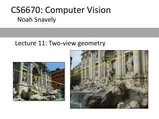
Overview of 2-view geometry. entering Part II of Hartley-Zissermanepipolar geometryformalization of the structure between 2 viewsused to extract depth information inherent in this stereo viewhow fundamental matrix F encodes epipolar geometrythe central structure in 2-view geometry is the fundam

E N D
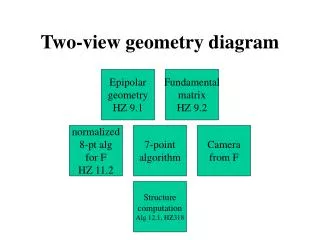
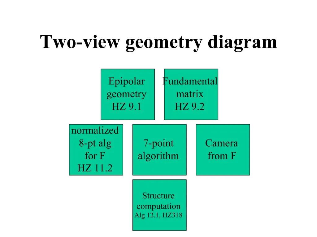
1. Two-view geometry diagram
2. Overview of 2-view geometry entering Part II of Hartley-Zisserman
epipolar geometry
formalization of the structure between 2 views
used to extract depth information inherent in this stereo view
how fundamental matrix F encodes epipolar geometry
the central structure in 2-view geometry is the fundamental matrix F: all of the camera and structure information is extracted directly or indirectly from F
solving for F using point correspondences
8 point algorithm
singularity constraint
normalization
7 point algorithm
how the fundamental matrix encodes the camera center and other camera information
3. Two-view geometry diagram
4. Finding structure imagine two cameras (perhaps virtually by moving a single camera in time)
camera centers c and c�
valid point correspondence (x,x�)
we want to discover the 3D point X associated with this point correspondence
finding X and finding c/c� are the main goals of structure from motion
we shall explore the geometric relationship between c,c�,x,x�,X
5. Epipolar geometry baseline = line cc� between camera centers; demo: cardboard, 2 frames
epipolar plane = any plane through the baseline
a pencil of planes
epipole = intersection of baseline with image plane
equivalently, image of other camera center
this connection to camera center will be leveraged
crucial to computing structure and camera
note: may lie outside image
epipolar line = intersection of an epipolar plane with an image plane
note: x has an associated epipolar plane (3 points define a plane), so an associated epipolar line
note: x� lies on the epipolar line associated with x
HZ239-241
6. Epipolar lines we have seen that x� lies on the x epipolar line, and x lies on the x� epipolar line
offers a mechanism to tie the two points together: if we can compute the epipolar line l� associated with a point x, then we have a constraint on the position of x�
l� . x� = 0 (x� lies on l�)
this tells us something about the companion x�
the fundamental matrix will build epipolar lines from points
so it is valuable in determining structure
epipolar line = image of cx line
7. Epipoles from epipolar lines epipolar lines are tied up with epipoles: epipole lies on every epipolar line
notice how the epipole can be found from these epipolar lines
this gives information about the other camera center
8. Fundamental matrix the fundamental matrix relates two images
the fundamental matrix F of two images is a 3x3 matrix such that:
F: points ? epipolar lines
Fx is the epipolar line (in image 2) associated with the point x (in image 1)
also vice versa using Ft: x� in image 2 => Ft x� in image 1
how do we interpret this? x is in a 2-space, Fx is in another 2-space
corollary: xtFx� = 0 if (x,x�) are a corresponding pair (i.e., image points of the same 3D point X)
proof: x lies on Fx�
F as epipolar line generator
F as correspondence checker
HZ242
9. Computing F: basics we will use xtFx� = 0 constraints from a few point correspondences to solve for F
each point pair (x,x�) defines a linear equation in F
8 pairs should be enough to solve for the 8 degrees of freedom in F (projective 3x3)
SIFT will be used to gather point correspondences
detailed algorithms below
10. Epipoles from F F yields information about the epipoles (on top of information about epipolar lines and point correspondences)
let e = epipole of image 1
e� = epipole of image 2
both are found as null spaces
Fe = 0
Ft e� = 0
proof below
11. Interpretation of F consider the epipolar line l� associated with x
l� = e� x x�
e� and x� lie on l�
so l� = [e�]x x�
skew-symmetric rep
but x� = Hx for some homography H
can be understood as point transfer off a plane, but not necessary
so l� = [e�]x Hx
we know l� = Fx, so:
F = [e�]x H
HZ243
12. Resulting properties of F F is rank 2
[e�]x is rank 2, H is rank 3
that is, F is singular and has 1d null space
adds a constraint that is very helpful in guiding the computation of F (see below)
proof that Fe = 0:
Fe = ([e�]x H) e = [e�]x (H e) = e� x (He) = e� x e� = 0
image of e is e�
thus, the epipole e may be found as the null space of F
13. CLAPACK OpenCV has SVD too
www.netlib.org/clapack/
download CLAPACK from www.netlib.org/clapack/clapack.tgz and www.netlib.org/clapack/clapack.h
install CLAPACK following www.netlib.org/clapack/readme.install
generates lapack_LINUX.a and blas_LINUX.a
optimize the BLAS for your machine (optional)
see my Makefile
see www.netlib.org/lapack for documentation
download the manual pages for ready access: e.g., once you discover through the search engine that �sgesv� solves Ax=b for you, �man sgesv� gives its parameters.
read CLAPACK/readme for caveats of style differences in calling LAPACK from C, such as column-major simulation and call by reference parameters.
sgesvd for SVD