Download
1 / 92
920 likes | 1.03k Views
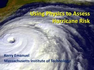
Using Physics to Help Assess Hurricane Risk. Kerry Emanuel Earth, Atmospheric, and Planetary Sciences Massachusetts Institute of Technology. Limitations of a strictly actuarial approach. Total Number of United States Landfall Events, by Category, 1870-2004.

E N D
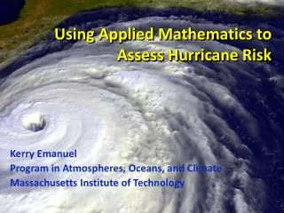
Using Physics to Help Assess Hurricane Risk Kerry Emanuel Earth, Atmospheric, and Planetary Sciences Massachusetts Institute of Technology
Total Number of United States Landfall Events, by Category, 1870-2004
U.S. Hurricane Damage, 1900-2004, Adjusted for Inflation, Wealth, and Population
Summary of U.S. Hurricane Damage Statistics: • >50% of all normalized damage caused by top 8 events, all category 3, 4 and 5 • >90% of all damage caused by storms of category 3 and greater • Category 3,4 and 5 events are only 13% of total landfalling events; only 30 since 1870 • Landfalling storm statistics are inadequate for assessing hurricane risk
Atlantic Sea Surface Temperatures and Storm Max Power Dissipation (Smoothed with a 1-3-4-3-1 filter) Years included: 1870-2006 Power Dissipation Index (PDI) Scaled Temperature Data Sources: NOAA/TPC, UKMO/HADSST1
Theoretical Upper Bound on Hurricane Maximum Wind Speed:POTENTIAL INTENSITY Surface temperature Ratio of exchange coefficients of enthalpy and momentum Outflow temperature Air-sea enthalpy disequilibrium
The Problem • The hurricane eyewall is a region of strong frontogenesis, attaining scales of ~ 1 km or less • At the same time, the storm’s circulation extends to ~1000 km and is embedded in much larger scale flows
Typhoon Megi 10/17/10 0457 GMT
Eyewall Undergoes Frontal Collapse • Will always challenge spatial resolution of numerical models • High resolution required for numerical convergence • Proper formulation of 3-D turbulence critical for adequate simulation of eyewall
Global Models do not simulate the storms that cause destruction! Modeled Histograms of Tropical Cyclone Intensity as Simulated by a Global Model with 50 km grid point spacing. (Courtesy Isaac Held, GFDL) Observed Category 3
Numerical convergence in an axisymmetric, nonhydrostatic model (Rotunno and Emanuel, 1987)
How to deal with this? • Option 1: Brute force and obstinacy
How to deal with this? • Option 1: Brute force and obstinacy • Option 2: Applied math and modest resources
Time-dependent, axisymmetric model phrased in R space • Hydrostatic and gradient balance above PBL • Moist adiabatic lapse rates on M surfaces above PBL • Boundary layer quasi-equilibrium convection • Deformation-based radial diffusion
Application to Real-Time Hurricane Intensity Forecasting • Must add ocean model • Must account for atmospheric wind shear
Ocean columns integrated only Along predicted storm track. Predicted storm center SST anomaly used for input to ALL atmospheric points.
Comparing Fixed to Interactive SST: Model with Fixed Ocean Temperature Model including Ocean Interaction
How Can We Use This Model to Help Assess Hurricane Risk in Current and Future Climates?
Risk Assessment Approach: Step 1: Seed each ocean basin with a very large number of weak, randomly located cyclones Step 2: Cyclones are assumed to move with the large scale atmospheric flow in which they are embedded, plus a correction for beta drift Step 3: Run the CHIPS model for each cyclone, and note how many achieve at least tropical storm strength Step 4: Using the small fraction of surviving events, determine storm statistics. Details: Emanuel et al., Bull. Amer. Meteor. Soc, 2008
Synthetic Track Generation:Generation of Synthetic Wind Time Series • Postulate that TCs move with vertically averaged environmental flow plus a “beta drift” correction • Approximate “vertically averaged” by weighted mean of 850 and 250 hPa flow
Synthetic wind time series • Monthly mean, variances and co-variances from re-analysis or global climate model data • Synthetic time series constrained to have the correct monthly mean, variance, co-variances and an power series
250 hPa zonal wind modeled as Fourier series in time with random phase: where T is a time scale corresponding to the period of the lowest frequency wave in the series, N is the total number of waves retained, and is, for each n, a random number between 0 and 1.
The time series of other flow components: or where each Fi has a different random phase, and A satisfies where COV is the symmetric matrix containing the variances and covariances of the flow components.Solved by Cholesky decomposition.
Track: Empirically determined constants:
Risk Assessment Approach: Step 1: Seed each ocean basin with a very large number of weak, randomly located cyclones Step 2: Cyclones are assumed to move with the large scale atmospheric flow in which they are embedded, plus a correction for beta drift Step 3: Run the CHIPS model for each cyclone, and note how many achieve at least tropical storm strength Step 4: Using the small fraction of surviving events, determine storm statistics. Details: Emanuel et al., Bull. Amer. Meteor. Soc, 2008
Comparison of Random Seeding Genesis Locations with Observations
6-hour zonal displacements in region bounded by 10o and 30o N latitude, and 80o and 30o W longitude, using only post-1970 hurricane data
Calibration Absolute genesis frequency calibrated to globe during the period 1980-2005
Genesis rates Western North Pacific Southern Hemisphere Eastern North Pacific Atlantic North Indian Ocean
Captures effects of regional climate phenomena (e.g. ENSO, AMM)
Seasonal Cycles Atlantic
Cumulative Distribution of Storm Lifetime Peak Wind Speed, with Sample of 1755Synthetic Tracks 95% confidence bounds
3000 Tracks within 100 km of Miami 95% confidence bounds