Download
1 / 28
310 likes | 790 Views
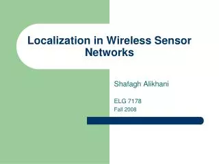
Localization in wireless sensor ad-hoc networks. Xiaobo Long ECSE 6962 course presentation. Introduction. What is localization Determine node locations in ad-hoc sensor networks Distributed Without relying on external infrastructure Without base stations, satellites, etc.

E N D
Localization in wireless sensor ad-hoc networks Xiaobo Long ECSE 6962 course presentation
Introduction • What is localization • Determine node locations in ad-hoc sensor networks • Distributed • Without relying on external infrastructure • Without base stations, satellites, etc. • GPS: too expensive • not suitable for low-cost, ad-hoc sensor networks • Why need localization • Routing techniques require knowledge of location • Sensing tasks require knowledge of location
Algorithms requirements • Truly distributed • employed on large-scale ad-hoc sensor networks • Self-organizing • do not depend on global infrastructure • Robust • be tolerant to node failures and range errors • Energy efficient • require little computation and communication
Assumptions • Nodes are randomly distributed • 2-D environment • Static network • Nodes don’t move • Anchor nodes • Have a priori knowledge of their own position • with respect to some global coordinate system
Important parameters • Range errors • describe accuracy of the distance measurements • effect accuracy of localization algorithms • Connectivity of the nodes • i.e., the average number of neighbors • Anchor fraction • some anchor nodes have a priori knowledge of their own position • Three context parameters are dependent
General algorithms [LR03]-Three phases • Distance to anchors • Determine the distances between unknowns and anchor nodes • starting at the anchor nodes, measure distance to neighbors • distance information is flooded into the network • flooding limit • three algorithms • Sum-dist • DV-hop • Euclidian • Node position • Derive for each node a position from its anchor distances • Lateration • Min–max • Refinement • Refine the node positions • using information about the range (distance) to, and positions of, neighboring nodes
Phase1: Distance to anchors • Sum-dist • adding the ranges at each hop during flooding • anchors nodes: • send a message • identity, position, and a path length set to 0 • receiving node: • adds the measured range to the path length • forwards (broadcasts) the message • if the flood limit allows • if the current path length is less than the previous one • result • each node have stored the position • minimum path length • drawbacks • range errors accumulate when distance information is propagated over multiple hops • error is significant for large networks with few anchors and/or poor ranging hardware
Distance to anchors (cont.) • DV-hop - use topological information instead of summing the (erroneous) ranges. • counting the number of hops • calibration: convert hop counts into distances • multiplying the hop count with an average hop distance • average hop distance obtained by anchors • drawback • fails for highly irregular network topologies • where the variance in actual hop distances is very large
Distance to anchors (cont.) • Euclidean • based on the local geometry of the nodes around an anchor • anchors: initiate a flood • receiver: • receive messages from two neighbors that: • know their distance to the anchor • know their distance to each other • calculate the distance to the anchor • result • two possible distance to anchor • solution • neighbor vote: a third neighbor n3 connected to either n1 or n2. replace n1 or n2 with n3
Phase 2: Node position • Nodes determine their position • based on the distance estimates to a number of anchors • provided by one of the three Phase 1 alternatives • Sum-dist, DV-hop, or Euclidean • Using: • the estimated distances (di) • known positions (xi; yi) • Methods • Lateration • Min–max
Lateration algorithm (1) unknown position is denoted by (x; y). (2) Linear the system by subtracting the last equation from the first n-1 equations. (3) Reordering the terms gives a proper system of linear equations in the form Ax = b (4) The system is solved using a standard least-squares approach: (5) additional sanity check by computing the residue between the given distances di and the distances to the location estimate of x (6) exceptional cases: the matrix inverse can not be computed and Lateration fails. * quite expensive in the number of floating point operations that is required.
Min–max algorithm • For each anchor: • construct a bounding box • using its position & distance to estimate • [xi-di, yi-di] x [xi+di, yi+di] • Determine the intersection of these boxes • [max(xi-di), max(yi-di)] x [min(xi+di), min(yi+di)] • Position of the node = center of the intersection box
Phase 3: Refinement • Refine the (initial) node positions computed during phase 2 • not all available information used in the first two phases • positions are not very accurate, even under good conditions • (high connectivity, small range errors) • Iterative refinement procedure • take into account all inter-node ranges • nodes update their positions • a node broadcasts its position estimate • receives the positions and range estimates from its neighbors • performs Lateration procedure of Phase 2 to determine its new position • refinement stops when position update becomes small -> reports the final position • Problem • errors propagate quickly through the network • a single error from 1 node needs only d iterations to affect all nodes (d: network diameter)
Examples of localization algorithms • Ad-hoc positioning by Niculescu and Nath [NN01] • Robust positioning by Savvides, Langendoen and Rabaey [SLR02] • N-hop multilateration by Savarese, Park and Srivastava [SPS02] • compare various alternatives for each phase • simulation on the same platform • conclusion • no single algorithm performs best • which algorithm be preferred depends on the conditions • range errors, connectivity, anchor fraction, etc. • still significant room for improving accuracy & increasing coverage
General problems for localization • insufficient data • lack of absolute reference points or anchors • distance measurements are noisy • creating additional uncertainty • difficult for scalability • algorithms that scale linearly with the size of the network are hard to devise • data must be broadcast through wireless channel • limited communications capacity.
Localization with Noisy Range Measurements [MLRT04] • Challenges of network localization with noise • only numerical optimization of distance constraints ---- fails • knowing the length of each graph edge ---- does NOT guarantee a unique realization • need to handle nodes with ambiguous positions • non-rigid graph • can be continuously deformed to produce an infinite number of different realizations • rigid graph • two kinds of ambiguity • flip ambiguities • discontinuous flex ambiguities • Can NOT be solved by graph rigidity theory or tests when distance measurements are noisy
Two kinds of ambiguity For (b): If edge AD is removed, then reinserted, the graph can flex in the direction of the arrow, taking on a different configuration but exactly preserving all distance constraints. For (a): Vertex A can be reflected across the line connecting B and C with no change in the distance constraints.
Solution for ambiguity problem • only localize those vertices that: • have a small probability of being flip or flex ambiguity • robust quadrilaterals • construct robust quadrilaterals regions to locate node • prevent incorrect realizations of flip ambiguities • would otherwise corrupt localization computations • cope with measurement noise in the system • drawback • bad performance under low node connectivity
Robust quadrilaterals algorithm • Define: cluster • a node and its set of neighbors • Three phases • Cluster localization • Quadrilaterals • the smallest possible sub-graph that can be unambiguously localized in isolation • identify all robust quadrilaterals • find the largest sub-graph • composed solely of overlapping robust quads • minimizes the probability of realizing a flip ambiguity • Cluster optimization (optional) • refine the position estimates for each cluster • using numerical optimization • Cluster transformation • compute transformations between neighboring clusters • finding the set of nodes in common between two clusters • solving for the rotation, translation, and possible reflection that best aligns the clusters
Quadrilaterals: • knowing the locations of any three vertices • sufficient to compute the location of the fourth using trilateration • problem • but still NOT sufficient to guarantee a unique graph realization • when distance measurements are noisy • If the smallest angle θi is near zero, there is a risk that measurement error • solution • restrict our quadrilateral to be robust ---> only those triangles with a sufficiently large minimum angle as robust • b is the length of the shortest side and θ is the smallest angle • use the robust quadrilateral as a starting point • localize additional nodes by chaining together connected robust quads • whenever two quads have three nodes in common & the first quad is fully localized • can localize the second quad by trilaterating from the three known positions
(a) robust four-vertex quadrilateral (b) decomposition of the robust quadrilateral into four triangles. If θ3 (smallest)is near zero: say in edge AD, will cause vertex D to be reflected over this sliver of a triangle
Localization with mere connectivity [SRZ03] • Goal • using fewer anchor nodes to derive the locations of the nodes • even yields relative coordinates when no anchor nodes are available • Method • MDS (multi-dimensional scaling) • starts with one or more distance matrices • derived from points in a multidimensional space • find a placement of the points in a low-dimensional space • usually two or three-dimensional • closely related to PCA (principal component analysis) • types of MDS techniques • classical metric MDS, replicated MDS, weighted MDS, etc. • Classical metric MDS • tolerates error gracefully • due to the over-determined nature of the solution • it can be performed efficiently on large matrices • a closed-form solution
MDS-MAP algorithm- Based on MDS • First step • estimate distance between each possible pair of nodes • use shortest-paths algorithm • shortest path distances are used to construct the distance matrix for MDS • Second step • apply classical MDS to the distance matrix • core of classical MDS • SVD (singular value decomposition) • result of MDS • a relative map that gives a location for each node • Third step • if given sufficient anchor nodes • transform the relative map to an absolute map • based on the absolute positions of anchors • Drawback • requires centralized computation
Localization for mobile sensor network [HE04] • Usually • mobility make localization more difficult • none of above mechanism consider mobile nodes and anchors • Sequential Monte Carlo localization • take advantage of mobility • to improve the accuracy of localization • reduce the number of anchors required • based on MCL (Monte Carlo Localization) • used for robots localization
Sequential Monte Carlo (SMC) • Key idea • estimate the posterior distribution of discrete time dynamic models • Algorithm • t: discrete time • l(t): position distribution of the node at time t • o(t): observations from anchor nodes received between time t-1 and time t • p(l(t) | l(t-1)): transition equation • prediction of node’s current position based on previous position • p(l(t) | o(t)): observation equation • describes the likelihood of the node being at the location l(t) given the observations • filter impossible positions • estimate recursively in time the filtering distribution p(l(t) | o(0), o(1), …, o(t)) • A set of N samples L(t) is used to represent the distribution l(t) • recursively computes the set of samples at each time step • since L(t-1) reflects all previous observations, can compute l(t) using only L(t-1) and o(t).
Conclusion • Goal • determine node locations in ad-hoc sensor networks • can use a small number of anchors • Three phases • various alternatives for each phase • Challenges • noisy distance measurements • mere connectivity • mobility
Reference • Ian F. Akyildiz, Weilian Su, Yogesh Sankarasubramaniam, and Erdal Cayirci, A Survey on Sensor Networks. • [LR02] Koen Langendoen, Niels Reijers, Distributed localization in wireless sensor networks: a quantitative comparison, Computer Networks, 2003, pp. 499-518. • [NN01] D. Niculescu, B. Nath, Ad-hoc positioning system, IEEE GlobeCom, 2001. • [SLR02] C. Savarese, K. Langendoen, J. Rabaey, Robust positioning algorithms for distributed ad-hoc wireless sensor networks, USENIX Technical Annual Conference, 2002, pp. 317–328. • [SPS02] A. Savvides, H. Park, M. Srivastava, The bits and flops of the N-hop multilateration primitive for node localization problems, in: First ACM International Workshop on Wireless Sensor Networks and Application (WSNA), 2002, pp. 112–121. • [MLRT04] David Moore, John Leonard, Daniela Rus and Seth Teller, Robust Distributed Network Localization with Noisy Range Measurements, ACM, 2004. • [SRZ03] Yi Shang, Wheeler Ruml, Ying Zhang, Markus P. J. Fromherz, Localization from Mere Connectivity, MobiHoc, 2003. • [HE04] Lingxuan Hu, David Evans, Localization for Mobile Sensor Networks, MobiCom, 2004.