Download
1 / 65
680 likes | 969 Views
The Chi-Square test. 2. Assistant prof. Dr. Mayasah A. Sadiq FICMS-FM. DATA. QUALITATIVE. QUANTITATIVE. CHI SQUARE TEST. T-TEST. The most obvious difference between the chi‑square tests and the other hypothesis tests we have considered (T test) is the nature of the data.

E N D
The Chi-Square test 2 Assistant prof. Dr. Mayasah A. Sadiq FICMS-FM
DATA QUALITATIVE QUANTITATIVE CHI SQUARE TEST T-TEST
The most obvious difference between the chi‑square tests and the other hypothesis tests we have considered (T test) is the nature of the data. • For chi‑square, the data are frequenciesrather than numerical scores.
Chi-squared Tests • For testing significance of patterns in qualitative data. • Test statistic is based on counts that represent the number of items that fall in each category • Test statistics measures the agreement between actual counts(observed) and expected counts assuming the null hypothesis
Applications of Chi-square test: • Goodness-of-fit • The 2 x 2 chi-square test (contingency table, four fold table) • The a x b chi-square test (r x c chi-square test)
Steps of CHI hypothesis testing • 1. Data :counts or proportion. • 2. Assumption: random sample selected from a population. • 3. HO :no sign. Difference in proportion • no significant association. • HA: sign. Difference in proportion • significant association.
4. level of sign. • df 1st application=k-1(k is no. of groups) • df 2nd &3rd application=(column-1)(row-1) • IN 2nd application(conengency table) • Df=1, tab. Chi= 3.841 always • Graph is one side (only +ve)
6. Statistical decision & 7. Conclusion • Calculated chi <tabulated chi • P>0.05 • Accept HO,(may be true) • If calculated chi> tabulated chi • P<0.05 • Reject HO& accept HA.
The Chi-Square Test for Goodness-of-Fit • The chi-square test for goodness-of-fit uses frequency data from a sample to test hypotheses about the shape or proportions of a population. • The data, called observed frequencies, simply count how many individuals from the sample are in each category.
Example • Eye colour in a sample of 40 • Blue 12,brown 21,green 3,others 4 • Eye colour in population • Brown 80% • Blue 10% • Green 2% • Others 8% • Is there any difference between proportion of sample to that of population .use α0.05
Expected counts(frequency) • Expected blue10/100*40=4 • Expected brown=80/100*40=32 • Expexcted green=2/100*40=0.8 • Expected others=8/100*40=3
1. Data • Represents the eye colour of 40 person in the following distribution • Brown=21 person,blue=12 person,green=3,others=4
2. Assumption • Sample is randomly selected from the population.
3. Hypothesis • Null hypothesis: there is no significant difference in proportion of eye colour of sample to that of the population. • Alternative hypothesis: there is significant difference in proportion of eye colour of sample to that of the population.
4. Level of significance; (α =0.05); • 5% Chance factor effect area • 95% Influencing factor effect area • d.f.(degree of freedom)=K-1; (K=Number of subgroups) • =4-1=3 • D.f. for 0.5=7.81
7.81 Accept Ho Influencing factor effect area 95% Reject Ho Chance factor effect area 5% 5%
Expected counts(frequency) • Expected blue=10/100*40=4 • Expected brown=80/100*40=32 • Expexcted green=2/100*40=0.8 • Expected others=8/100*40=3
=(12-4)² (21-32)² (3-0.8)² (4-3)² • ------------ +---------- +----------- + -------- • 4 32 0.8 3 • =(64/4) + (121/32)+(4.8/0.8)+(1/3) • =16+3.78+6+0.3= • Calculated chi =26.08
7.81 Accept Ho Influencing factor effect area 95% Reject Ho Chance factor effect area 5% 5%
6. Statistical decision • Calculated chi> tabulated chi • P<0.5
7. Conclusion • We reject H0 &accept HA: there is significant difference in proportion of eye colour of sample to that of the population.
Applications of Chi-square test: • Goodness-of-fit • The 2 x 2 chi-square test (contingency table, four fold table) • The a x b chi-square test (r x c chi-square test)
The Chi-Square Test for Independence • The second chi-square test, the chi-square test for independence, can be used and interpreted in two different ways: 1. Testing hypotheses about the relationship between two variables in a population, or(2×2) 2. Testing hypotheses about differences between proportions for two or more populations.(a×b)
The Chi-Square Test for Independence (cont.) • The data, called observed frequencies, simply show how many individuals from the sample are in each cell of the matrix. • The null hypothesis for this test states that there is no relationship between the two variables; that is, the two variables are independent.
The Chi-Square Test for Independence (cont.) The calculation of chi-square is the same for all chi-square tests:
Example • A total 1500 workers on 2 operators(A&B) • Were classified as deaf & non-deaf according to the following table.is there association between deafness & type of operator .let α 0.05
Result notdeaf. total deaf Operator A 100 900 1000 B 60 440 500 total 160 1340 1500
Result notdeaf. total deaf Operator A 100 900 1000 B 60 440 500 total 160 1340 1500 Total number of items=1500 Total number of defective items=160
Result notdef. total def Operator A 100 900 1000 B 60 440 500 total 160 1340 1500 Expected deaf from Operator A = 1000 * 160/1500 = 106.7 (expected not deaf=1000-106.7=893.3) Expected deaf from Operator B = 500 * 160/1500 = 53.3
notdef. total def Operator 1000 A 100 900 B 60 440 500 total 160 1340 1500 Expected notdef. total def Operator A 106.7 893.3 B 53.3 446.7 total Result
1. Data • Represent 1500 workers,1000 on operator A 100 of them were deaf while 500 on operator B 60 of them were deaf
2. Assumption • Sample is randomly selected from the population.
3. Hypothesis • HO: there is no significant association between type of operator & deafness. • HA:there is significant association between type of operator & deafness.
4. Level of significance; (α = 0.05); • 5% Chance factor effect area • 95% Influencing factor effect area • d.f.(degree of freedom)=(r-1)(c-1) =(2-1)(2-1)=1 • D.f. 1 for 0.05=3.841
3.841 Accept Ho Influencing factor effect area 95% Reject Ho Chance factor effect area 5% 5%