Download
1 / 19
200 likes | 675 Views
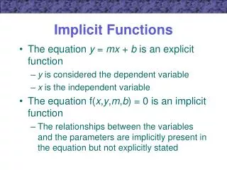
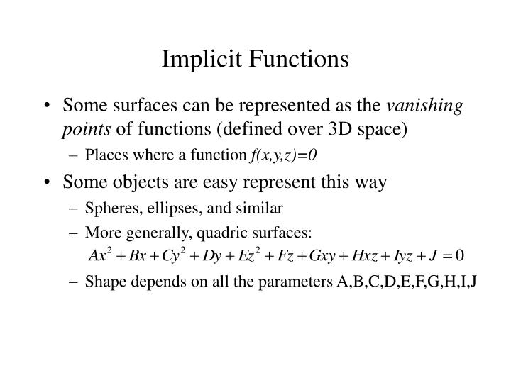
Implicit Functions. Some surfaces can be represented as the vanishing points of functions (defined over 3D space) Places where a function f(x,y,z)=0 Some objects are easy represent this way Spheres, ellipses, and similar More generally, quadric surfaces:

E N D
Implicit Functions • Some surfaces can be represented as the vanishing points of functions (defined over 3D space) • Places where a function f(x,y,z)=0 • Some objects are easy represent this way • Spheres, ellipses, and similar • More generally, quadric surfaces: • Shape depends on all the parameters A,B,C,D,E,F,G,H,I,J
Blobs and Metaballs • Define the location of some points • For each point, define a function on the distance to a given point, (x,y,z) • Sum these functions up, and use them as an implicit function • Question: If I have two special points, in 2D, and my function is just the distance, what shape results? • More generally, use gaussian functions of distance, or other forms • Various results are called blobs or metaballs
Rendering Implicit Surfaces • Some methods can render then directly • Raytracing - find intersections with Newton’s method • For polygonal renderer, must convert to polygons • Advantages: • Good for organic looking shapes eg human body • Reasonable interfaces for design • Disadvantages: • Difficult to render and control when animating • Being replaced with subdivision surfaces, it appears
Production Rules • Model by giving a set of rules to follow to generate it • Works best for things like plants: • Start with a stem • Replace it with stem + branches • Replace some part with more stem + branches, and so on • Essentially, generate a string that describes the object by replacing sub-strings with new sub-strings • Render by generating geometry • Parametric instances of branch, leaf, flower, etc • Or polygons, or blobs, or … • Can work for whole gardens and forests
L-Systems Generator Prusinkiewicz, Hammel, Mech http://www.cpsc.ucalgary.ca/projects/bmv/vmm/title.html
L-Systems Prusinkiewicz, Hammel, Mech http://www.cpsc.ucalgary.ca/projects/bmv/vmm/title.html
More L-Systems Prusinkiewicz, Hammel, Mech http://www.cpsc.ucalgary.ca/projects/bmv/vmm/title.html
Yet More L-systems Prusinkiewicz, Hammel, Mech http://www.cpsc.ucalgary.ca/projects/bmv/vmm/title.html
Shortcomings • The representations we have looked at so far have various failings: • Meshes are large, difficult to edit, require normal approximations, … • Parametric instancing has a limited domain of shapes • CSG is difficult to render and limited in range of shapes • Implicit models are difficult to control and render • Production rules work in highly limited domains • Parametric curves and surfaces address many of these issues • More general than parametric instancing • Easier to control than meshes and implicit models
Parametric Curves • We have seen the parametric form for a line: • Note that x, y and z are each given by one equation that involves: • The parameter t • Some user specified control points, x0 and x1 • This is an example of a parametric curve
Hermite Spline • A spline is a parametric curve defined by some control points • The term spline dates from engineering drawing, where a spline was a piece of flexible wood used to draw smooth curves • The control points are adjusted by the user to control the shape of the curve • A Hermite spline is typically a cubic curve for which the user provides: • The endpoints of the curve • The parametric derivatives of the curve at the endpoints • The parametric derivatives are dx/dt, dy/dt, dz/dt
Hermite Spline (2) • Say the user provides • A cubic spline has degree 3, and is of the form: • For some constants a, b, c and d derived from the control points, but how? • We have constraints: • The curve must pass through x0 when t=0 • The derivative must be x’0 when t=0 • The curve must pass through x1 when t=1 • The derivative must be x’1 when t=1
Hermite Spline (3) • Solving for the unknowns gives: • Rearranging gives: or
Basis Functions • A point on a Hermite curve is obtained by multiplying each control point by some function and summing • The functions are called basis functions
Bezier Curves (1) • Different choices of basis functions give different curves • Choice of basis determines how the control points influence the curve • In Hermite case, two control points define endpoints, and two more define parametric derivatives • For Bezier curves, two control points define endpoints, and two control the tangents at the endpoints in a geometric way
Bezier Curves (2) • The user supplies 4 control points, pi • Write the curve as: • The functions Bd are the Bernstein polynomials of degree d • This equation can be written as a matrix equation also • There is a matrix to take Hermite control points to Bezier control points
Bezier Curve Properties • The first and last control points are interpolated • The tangent to the curve at the first control point is along the line joining the first and second control points • The tangent at the last control point is along the line joining the second last and last control points • The curve lies entirely within the convex hull of its control points • The Bernstein polynomials (the basis functions) sum to 1 • They can be rendered in many ways • Convert to line segments with a subdivision algorithm