Understanding Short-Time Fourier Transform: Theory and Implementations

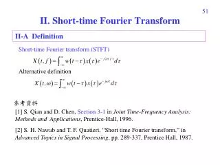
1. INTRODUCTION TO THESHORT-TIME FOURIER TRANSFORM (STFT) Richard M. Stern, Raymond Xia 18-491 lecture April 22, 2019 Department of Electrical and Computer Engineering Carnegie Mellon University Pittsburgh, Pennsylvania 15213

2. Why consider short-time Fourier transforms? • Conventional DTFT sums over all time: • An example: “Welcome to DSP-I” • The DTFT averages frequency components over time • (from the creation of the universe until ???}

3. “Welcome to DSP-I” in time and frequency

4. Why we want the STFT … • We are more interested in how the frequency components of real sounds like speech and music vary over time • Example: the spectrogram of “Welcome to DSP-I”

5. The direct (Fourier transform) approach to STFTs • Multiply the time function and by a sliding window, and take the DTFT of the product: • Comments: • Note that m is a dummy variable and that the window is time-reversed • Notation is consistent with chapter by Nawab and Quatieri in book edited by Lim and Oppenheim; OSPY notation is a little different • Results are plotted as a vector function of n, which is called the index of the analysis frame • Windows most commonly used are Hamming, rectangular, and exponential

6. An example with exponential windowing

7. Impact of window size and shape • The DTFT of the window is • Letting l = m–n and m = n–l, we obtain • Hence … • The STFT can be thought of as the circular convolution in frequency of the DTFT of x[m] with the DTFT of w[n–m]

8. Effect of window duration • The window duration mediates the tradeoff between resolution in time and frequency: • Short-duration window: Long-Duration window: • Best choice of window duration depends on the application

9. Can the STFT be inverted? • Yes, but …. • Consider the STFT as the transform of the windowed time function: • For n=m we can write • Or, of course • So the only absolute constraint for inversion is

10. The discrete STFT • Normally we would like the STFT to be discrete in frequency as well as time (for practical reasons) • We use which is evaluated at

11. Summary: the Fourier transform implementation of the STFT • The Fourier transform implementation of the STFT: • Window input function • Take Fourier transform • Repeat, after shifting window

12. There are other ways of computing the STFT! • Again, the STFT equation is • Rearranging the terms, we obtain the convolution • This can expressed as the lowpass implementation of the STFT:

13. The lowpass implementation of the STFT • Note that the frequency response of practical windows w[n] is almost invariably that of a lowpass filter • The lowpass implementation translates the spectrum of x[n] to the left by radians and passes through a lowpass filter

14. The Hamming window as a lowpass filter • The width of the main lobe of a Hamming window is • We will think of it as if it were an ideal LPF with the same bandwidth Spectrum of Hamming window, M = 40 Approximated ideal rectangular spectrum Single-sided BW is 4π/M

15. Also, the bandpass implementation of the STFT • The original STFT equation remains • Pre-multiplying and post-multiplying by produces • Which can be expressed as the bandpass implementation of the SFFT:

16. The bandpass implementation of the STFT • The bandpass implementation can be thought of as passing the signal through a (single-channel) bandpass filter and then shifting the output down to “baseband” • All three implementations are mathematically equivalent representations of the STFT • The signal at the output of the BPF has the same magnitude as X[n,k] but different phase

17. Some additional comments on implementations • In the Fourier transform implementation will develop the STFT on a column-by-column (or time frame by time frame) basis • In the LP and BP implementations we work on a row-by-row (or frequency-by-frequency) basis • Because the STFT is lowpass in nature, it can be downsampled. The downsampling ratio depends on the size and shape of the window.

18. Reconstructing the time function • Two major methods used: • Filterbank summation (FBS), based on LP and BP implementations • Overlap-add (OLA), based on the Fourier transform implementation

19. Reconstructing the time function using FBS • Filterbank summation: • Multiply each channel by • Add channels together and • multiply by a constant • This will work if all filters • add to a constant in frequency

20. The overlap-add (OLA) method of reconstruction • Procedure: • Compute the IDTFT for each column of the STFT • Add the IDTFTs together in the locations of the original window locations • The OLA resynthesis approach will work if all of the windows add up to a constant. Two (of many) solutions: • Abutting rectangular windows • Hamming windows spaced by 50% of their length

21. How many numbers do we need to keep? • The answer depends on the method used for analysis and synthesis. • For the Fourier transform STFT analysis with OLA resynthesis: • Need at least N samples in frequency for windows of length N (as is always true for DFTs) • The analysis frames can be separated by N samples for rectangular windows or N/2 samples for Hamming windows • This means that the total number of STFT coefficients per second needed will be NFs/N = Fs for rectangular windows or NFs/(N/2) for Hamming windows • Hence, the STFT requires the same or double the number of numbers in the original waveform. (And these numbers are complex!) We accept this for the benefits that STFTs provide

22. Summary • Short-time Fourier transforms enable us to analyze how frequency components evolve over time. The most straightforward approach is to window the time function and compute the DFT • The duration of the window mediates temporal versus spectral resolution • The original waveform can be resynthesized from the STFT representation • The number of numbers needed for the representation is somewhat greater, but that is a small price to pay for the ability to analyze and manipulate the input.