Download
1 / 38
400 likes | 1.14k Views
Testing Statistical Hypothesis The One Sample t-Test. Heibatollah Baghi, and Mastee Badii. Parametric and Nonparametric Tests. Parametric tests estimate at least one parameter (in t-test it is population mean)

E N D
Testing Statistical HypothesisThe One Sample t-Test Heibatollah Baghi, and Mastee Badii
Parametric and Nonparametric Tests • Parametric tests estimate at least one parameter (in t-test it is population mean) Usually for normal distributions and when the dependent variable is interval/ratio • Nonparametric tests do not test hypothesis about specific population parameters Distribution-free tests Although appropriate for all levels of measurement most frequently applied for nominal or ordinal measures
Parametric and Nonparametric Tests • Nonparametric tests are easier to compute and have less restrictive assumptions • Parametric tests are much more powerful (less likely to have type II error) What is type two error? This lecture focuses on One sample t-test which is a parametric test
Two Types of Error • Alpha: α • Probability of Type I Error • P (Rejecting Ho when Ho is true) • Predetermined Level of significance • Beta: β • Probability of Type II Error • P (Failing to reject Ho when Ho is false)
True False True (Accept Ho) Type II error Probability = b False (Rejects Ho) Type I error Probability = a Types of Error in Hypothesis Testing Ho: Hand-washing has no effect on bacteria counts
True False True (Accept Ho) Correct decision Probability = 1- a Type II error Probability = b False (Rejects Ho) Type I error Probability = a Correct decision Probability = 1- b Types of Error in Hypothesis Testing Ho: Hand-washing has no effect on bacteria counts
True False True (Accept Ho) Correct decision Probability = 1- a Type II error Probability = b False (Rejects Ho) Type I error Probability = a Correct decision Probability = 1- b Power & Confidence Level • Power • 1- β • Probability of rejecting Ho when Ho is false • Confidence level • 1- α • Probability of failing to reject Ho when Ho is true
Level of Significance • α is a predetermined value by convention usually 0.05 • α = 0.05 corresponds to the 95% confidence level • We are accepting the risk that out of 100 samples, we would reject a true null hypothesis five times
Population of IQ scores, 10-year olds µ=100 σ=16 n = 64 Sample 1 Sample 2 Sample 3 Etc Sampling Distribution Of Means
Sampling Distribution Of Means • A sampling distribution of means is the relative frequency distribution of the means of all possible samples of size n that could be selected from the population.
One Sample Test • Compares mean of a sample to known population mean • Z-test • T-test This lecture focuses on one sample t-test
The One Sample t – Test Testing statistical hypothesis about µ when σ is not known OR sample size is small
An Example Problem • Suppose that Dr. Tate learns from a national survey that the average undergraduate student in the United States spends 6.75 hours each week on the Internet – composing and reading e-mail, exploring the Web and constructing home pages. Dr. Tate is interested in knowing how Internet use among students at George Mason University compares with this national average. • Dr. Tate randomly selects a sample of only 10 students. Each student is asked to report the number of hours he or she spends on the Internet in a typical week during the academic year. Population mean Small sample Population variance is unknown & estimated from sample
Steps in Test of Hypothesis • Determine the appropriate test • Establish the level of significance:α • Determine whether to use a one tail or two tail test • Calculate the test statistic • Determine the degree of freedom • Compare computed test statistic against a tabled value
1. Determine the appropriate test • If sample size is more than 30 use z-test • If sample size is less than 30 use t-test • Sample size of 10
2. Establish Level of Significance • α is a predetermined value • The convention • α = .05 • α = .01 • α = .001 • In this example, assume α = 0.05
3. Determine Whether to Use a One or Two Tailed Test • H0 :µ = 6.75 • Ha :µ ≠ 6.75 A two tailed test because it can be either larger or smaller
4. Calculating Test Statistics Sample mean
4. Calculating Test Statistics Deviation from sample mean
4. Calculating Test Statistics Squared deviation from sample mean
4. Calculating Test Statistics Standard deviation of observations
4. Calculating Test Statistics Calculated t value
4. Calculating Test Statistics Standard deviation of sample means
4. Calculating Test Statistics Calculated t
5. Determine Degrees of Freedom • Degrees of freedom, df, is value indicating the number of independent pieces of information a sample can provide for purposes of statistical inference. • Df = Sample size – Number of parameters estimated • Df is n-1 for one sample test of mean because the population variance is estimated from the sample
Degrees of Freedom • Suppose you have a sample of three observations: X -------- -------- --------
Degrees of Freedom • Why n-1 and not n? • Are these three deviations independent of one another? • No, if you know that two of the deviation scores are -1 and -1, the third deviation score gives you no new independent information ---it has to be +2 for all three to sum to 0.
Degrees of Freedom Continued • For your sample scores, you have only two independent pieces of information, or degrees of freedom, on which to base your estimates of S and
6. Compare the Computed Test Statistic Against a Tabled Value • α = .05 • Df = n-1 = 9 • Therefore, reject H0
Decision Rule for t-Scores If |tc| > |tα| Reject H0
Decision Rule for P-values If p value < α Reject H0 Pvalue is one minus probability of observing the t-value calculated from our sample
Example of Decision Rules • In terms of t score: |tc = 2.449| > |tα= 2.262| Reject H0 • In terms of p-value: If p value = .037 < α = .05 Reject H0
Constructing a Confidence Interval for µ Standard deviation of sample means Sample mean Critical t value
Constructing a Confidence Interval for µ for the Example • Sample mean is 9.90 • Critical t value is 2.262 • Standard deviation of sample means is 1.29 • 9.90 + 2.262 * 1.29 • The estimated interval goes from 6.98 to 12.84
Distribution of Mean of Samples In drawing samples at random, the probability is .95 that an interval constructed with the rule will include m
Sample Report of One Sample t-test in Literature One Sample t-test Testing Neutrality of Attitudes Towards Infertility Alternatives
N Mean Std. Deviation Std. Error Mean Number of Hours 10 9.90 4.067 1.286 Test Value = 6.75 tc df Sig. (2-tailed) Mean Difference 95% Confidence Interval of the Difference Lower Upper Number of Hours 2.449 9 .037 3.150 .24 6.06 Testing Statistical Hypothesis With SPSS SPSS Output: One-Sample Statistics One-Sample Test
Take Home Lesson Procedures for Conducting & Interpreting One Sample Mean Test with Unknown Variance