Download
1 / 22
220 likes | 308 Views
Emergence of patterns in the geologic record and what those patterns can tell us about Earth surface processes. Hydrologic Synthesis Reverse Site Visit – August 20, 2009. Rina Schumer Desert Research Institute, Reno NV, USA. Water Cycle Dynamics. Hydrosphere/ Biosphere. Hillslopes.

E N D
Emergence of patterns in the geologic record and what those patterns can tell us about Earth surface processes Hydrologic Synthesis Reverse Site Visit – August 20, 2009 Rina Schumer Desert Research Institute, Reno NV, USA
Water Cycle Dynamics Hydrosphere/ Biosphere Hillslopes Transport of water/sediment/biota over heterogeneous surfaces How can we improve predictability? Synthesis subgroup #5 Stochastic Transport and Emergent Scaling in Earth-Surface Processes (STRESS)
Synthesis (Carpenter et al., 2009 - BioScience) • Sustained, intense interaction among individuals with ready access to data: • mine existing data from new perspectives that allow novel analyses • develop and use new analytical/computation/modeling tools that may lead to greater insights • bring theoreticians, empiricists, modelers, practitioners together to formulate new approaches to existing questions • integrate science with education and real-world problems
STRESS working group 2007-2009 Results of Synthesis “acceleration of innovation” gravel transport sediment transport in sand bed rivers non-local transport on hillslopes bedform deformation solute transport in streams ~2000 sediment accumulation rates solute transport in groundwater flow systems 1990’s depositional fluvial profiles slope-dependent soil transport hillslope evolution flow through heterogeneous hillslopes landslide geometry and debris mobilization Timeline showing use of heavy-tailed stochastic processes in modeling Earth surface systems transport on river networks
Introduction • Geology records the “noisiness" of sediment transport, as seen in wide range of sizes of sedimentary bodies • intermittency at many scales • Describe nature and pace of landscape evolution by separating random transport from forcing mechanisms (glacial cycles,tectonics,etc) • Need to estimate deposition rate
hiatus Influence of transport fluctuations on stratigraphy Modified from Sadler 1999
Shoreline LOG (Accumulation rate) [mm/yr] 7 Shelf Delta 6 Continental Rise 5 Abyssal Plain 4 -3/4 3 2 1 0 -1 -1/5 -2 -3 -6 -5 -4 -3 -2 -1 0 1 2 3 4 5 6 7 8 LOG (Time interval, t ) [yr] measured deposition rate depends on measurement interval “Sadler Effect” accumulation rate = thickness/time 1,000 yr. hiatus 500 yr. hiatus 100 yr. hiatus 1,000 yr. hiatus 50 yr. hiatus 2,000 yr. hiatus 40,000 yr. hiatus 1,000 yr. hiatus 10 yr. hiatus 1,000 yr. hiatus
Shoreline LOG (Accumulation rate) [mm/yr] 7 Shelf Delta 6 Continental Rise 5 Abyssal Plain 4 3 -3/4 2 1 0 -1 -2 -3 -6 -5 -4 -3 -2 -1 0 1 2 3 4 5 6 7 8 LOG (Time interval, t ) [yr] measured deposition rate depends on measurement interval “Sadler Effect” accumulation rate = thickness/time 1,000 yr. hiatus 500 yr. hiatus 100 yr. hiatus 1,000 yr. hiatus 50 yr. hiatus 2,000 yr. hiatus 40,000 yr. hiatus -1/5 1,000 yr. hiatus 10 yr. hiatus 1,000 yr. hiatus
Shoreline LOG (Accumulation rate) [mm/yr] 7 Shelf Delta 6 Continental Rise 5 Abyssal Plain 4 3 -3/4 2 1 0 -1 -2 -3 -6 -5 -4 -3 -2 -1 0 1 2 3 4 5 6 7 8 LOG (Time interval, t ) [yr] measured deposition rate depends on measurement interval “Sadler Effect” accumulation rate = thickness/time 1,000 yr. hiatus 500 yr. hiatus 100 yr. hiatus 1,000 yr. hiatus 50 yr. hiatus 2,000 yr. hiatus 40,000 yr. hiatus -1/5 1,000 yr. hiatus 10 yr. hiatus 1,000 yr. hiatus
Shoreline LOG (Accumulation rate) [mm/yr] 7 Shelf Delta 6 Continental Rise 5 Abyssal Plain 4 3 -3/4 2 1 0 -1 -2 -3 -6 -5 -4 -3 -2 -1 0 1 2 3 4 5 6 7 8 LOG (Time interval, t ) [yr] measured deposition rate depends on measurement interval “Sadler Effect” accumulation rate = thickness/time 1,000 yr. hiatus 500 yr. hiatus 100 yr. hiatus 1,000 yr. hiatus 50 yr. hiatus 2,000 yr. hiatus 40,000 yr. hiatus -1/5 1,000 yr. hiatus 10 yr. hiatus 1,000 yr. hiatus >350 references to Sadler(1981) !
Shoreline LOG (Accumulation rate) [mm/yr] 7 Shelf Delta 6 Continental Rise 5 Abyssal Plain 4 -3/4 3 2 1 0 -1/5 -1 -2 -3 -6 -5 -4 -3 -2 -1 0 1 2 3 4 5 6 7 8 LOG (Time interval, t ) [yr] “Sadler Effect” Attributed to (Sadler, 1981) • Strong correlation between sample age and measurement interval • Young samples small interval • Old samples long intervals • No constant sampling intervals • Greater probability of encountering a long hiatus in a longer interval: const
Shoreline LOG (Accumulation rate) [mm/yr] 7 Shelf Delta 6 Continental Rise 5 Abyssal Plain 4 -3/4 3 2 1 0 -1/5 -1 -2 -3 -6 -5 -4 -3 -2 -1 0 1 2 3 4 5 6 7 8 LOG (Time interval, t ) [yr] Our Conclusions • Sadler effect will arise if the length of hiatus periods follow a probability distribution with infinite mean • (aka power-law*, heavy-tailed) • Log-log slope of the Sadler plot is directly related to the tail of the hiatus length density *power law suggested previously by Plotnick, 1986 and Pelletier, 2007
Exponential (mean=10) Pareto (tail parameter=0.8) running mean running mean number of random variables number of random variables Infinite-mean probability density
No hiatus periods Incorporate avg. fraction of time with no deposition Measured accumulation rate Robs S(t2) S(t1) What if there is no average size hiatus because there is always a finite probability of intersecting a larger hiatus?
CTRW – discrete stochastic model random # of events by time t is a function of the hiatus lengths J8 Y7 J7 Y6 J6 J5 Y5 Y4 J4 J3 Y3 sediment accumulationevent length location of Sediment surface Y2 J2 Y1 T1 T2 T3 T4 T5 T6 T7
Governing equations for scaling limits of CTRW scaling limit CTRW Governing Equation Constant jump length Random hiatus length with thin tails Advection equation with retardation Constant jump length Random hiatus length with heavy tails Time-fractional advection equation S(t)= surface location with time, R=deposition rate, b=retardation coeff.
sediment surface elevation (mm) time (yr) Expected location of sediment surface with time analytical and numerical modelling: CTRW with constant (small) depostional periods, random hiatus length NO heavy tails in hiatus density heavy tails in hiatus density sediment surface elevation (mm) time (yr)
Sadler effect arises from heavy tailed hiatus distribution analytical and numerical modelling: CTRW with constant (small) depostional periods, random hiatus length NO heavy tails in hiatus density heavy tails in hiatus density Observed deposition rate (mm) observed deposition rate (mm/yr) convergence to constant time (yr) time (yr)
No hiatus periods Incorporate avg. fraction of time with no deposition Measured accumulation rate Robs S(t2) S(t1) Incorporate heavy tailed hiatuses A power-law function of time
30 Sediment mass [x 1018 kg] 25 20 15 10 5 0 10 20 30 40 50 60 Age [Ma] Implications: Measurement bias or…..climate change? Erosionrate [km3/Myr] Global values for terrigenous sediment accumulation (after Hay 1988 and Molnar 2004) • Same patterns seen in rate measurements for Age [Ma] Eastern Alps volumetric erosion rates estimated from surrounding basin accumulation rates (adapted from Kuhlemann et al. 2001) • subsidence • erosion • incision • evolution!
Synthesis (Carpenter, et al. BioScience) • Sustained, intense interaction among individuals with ready access to data: • mine existing data from new perspectives that allow novel analyses • develop and use new analytical/computation/modeling tools that may lead to greater insights • bring theoreticians, empiricists, modelers, practitioners together to formulate new approaches to existing questions • integrate science with education and real-world problems
References Hay, W.W., J.L. Sloan, and C.N. Wold (1988). Mass/Age distribution and composition of sediments on the ocean floor and the global rate of sediment subduction. J. Geophys. Res., 93(B12), 14933-14940. Molnar, P. (2004) Late Cenozoic increase in accumulation rates of terrestrial sediment: How might climate change have affected erosion rates?, Annual Review of Earth and Planetary Sciences, 32, 67-89. Pelletier, J.D. (2007) Cantor set model of eolian dust deposits on desert alluvial fan terraces, Geology, 35, 439-442. Plotnick, R.E. (1986) A fractal model for the distribution of stratigraphic hiatuses, J. Geology, 94(6), 885-890. Sadler, P.M. (1981) Sediment accumulation rates and the completeness of stratigraphic sections, J. Geology, 89(5), 569-584. Sadler, P.M. (1999) The influence of hiatuses on sediment accumulation rates, GeoRes. Forum,5, 15-40.