Download
1 / 34
350 likes | 475 Views
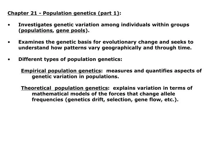
Chapter 21 - Population genetics (part 1) : Investigates genetic variation among individuals within groups ( populations , gene pools ). Examines the genetic basis for evolutionary change and seeks to understand how patterns vary geographically and through time.

E N D
Chapter 21 - Population genetics (part 1): • Investigates genetic variation among individuals within groups (populations, gene pools). • Examines the genetic basis for evolutionary change and seeks to understand how patterns vary geographically and through time. • Different types of population genetics: • Empirical population genetics: measures and quantifies aspects of genetic variation in populations. • Theoretical population genetics: explains variation in terms of mathematical models of the forces that change allele frequencies (genetics drift, selection, gene flow, etc.).
Types of questions studied by population geneticists: • How much variation occurs in natural populations, and what processes control the variation observed? • How does geography and dispersal behavior shape population structure? • What forces are responsible for population differentiation and how do they affect genetic diversity? • Mutation genetic diversity • Selection genetic diversity • Genetic drift genetic diversity • Migration genetic diversity • Non-random mating genetic diversity • Recombination genetic diversity • How do these forces and processes relate to Hardy-Weinberg Equilibrium assumptions? • How do demographic factors such as breeding system, fecundity, changes in population size, and age structure influence the gene pool in the population?
Population genetics: • One of the oldest and richest examples of success of mathematical theory in biology. • Provided synthesis of Mendelian genetics and Darwinian natural selection in the first part of the 20th century “modern synthesis”. • Modern synthesis is the foundation for modern evolutionary biology and population genetics.
Laid the first early groundwork the modern synthesis: Charles Darwin 1809-1882 The Origin of Species Alfred Russell Wallace 1823-1913 “Wallace’s Line” Thomas H. Huxley 1825-1895 “Darwin’s Bulldog”
Theoretical/mathematical population geneticists: Ronald A. Fisher 1890-1962 The Genetical Theory of Natural Selection J. B. S. Haldane 1892-1964 The Causes of Evolution Sewall Wright 1889-1988 Evolution and the Genetics of Populations - 4 vol.
Architects the modern synthesis, extended theoretical work of Fisher, Haldane, and Wright to real organisms: Theodosius Dobzhansky 1900-1975 Genetics and the Origin of Species Julian Huxley 1887-1975 Evolution: The Modern Synthesis Ernst Mayr 1904-2005 Systematics and the Origin of Species “Biological Species Concept” George G. Simpson 1902-1984 Tempo and Mode in Evolution George L. Stebbins 1906-2000 Variation and Evolution in Plants
Important topics within population genetics: • Today and next lecture • Genetic structure of populations • Hardy-Weinberg Equilibrium • Genetic variation in space and time • Variation in natural populations, Wright’s Fixation Index (Fst) • Forces that change gene frequencies
Ways to describe genetic structure of populations: • Genotypic frequency • Count individuals with one genotype and divide by total number of individuals. Repeat for each genotype in the population: • f(BB) = 452/497 = 0.909 • f(Bb) = 43/497 = 0.087 • f(bb) = 2/497 = 0.004 • Total = 1.000
Ways to describe genetic structure of populations: • Allelic frequency • Allelic frequencies offer more information than genotypic frequencies and can be calculated in two different ways: • Allele (gene) counting method: p = f(A) = (2 x count of AA) + (1 count of Aa)/ 2 x total number of individuals • Genotypic frequency method: p = f(A) = (frequency of the AA homozygote) + (1/2 x frequency of the Aa heterozygote) p = f(a) = (frequency of the aa homozygote) + (1/2 x frequency of the Aa heterozygote)
Allelic frequencies with multiple alleles: • Example: A1, A2, and A3 • p = f(A1) = (2 x A1A1) + (A1A2) + (A1A3)/2 x total individuals • q = f(A2) = (2 x A2A2) + (A1A2) + (A2A3)/2 x total individuals • r = f(A3) = (2 x A3A3) + (A1A3) + (A2A3)/2 x total individuals • Or • p = f(A1) = f(A1A1) +f(A1A2)/2 + f(A1A3)/2 • q = f(A2) = f(A2A2) + f(A1A2)/2 + f(A2A3)/2 • r = f(A3) = f(A3A3) + f(A1A3)/2 + f(A2A3)/2
Allelic frequencies at X-linked loci: • Females have 2 X-linked alleles, and males have 1 X-linked allele. • p = f(XA) = (2 x XA XA females) + (XA Xa females) + (XA Y males)/ • (2 x # females) + (# males) • q = f(Xa) = (2 x Xa Xa females) + (XA Xa females) + (Xa Y males)/ • (2 x # females) + (# males) • If number of females and males are equal: • p = f(XA) = 2/3[f(XAXA) +1/2f(XAXa)] + 1/3f(XAY) • q = f(Xa) = 2/3[f(XaXa) +1/2f(XAXa)] + 1/3f(XaY)
Hardy-Weinberg law: • Independently discovered by Godfrey H. Hardy (1877-1947) and Wilhelm Weinberg (1862-1937). • Explains how Mendelian segregation influences allelic and genotypic frequencies in a population. • Assumptions: • Population is infinitely large, to avoid effects of genetic drift (= change in genetic frequency due to chance). • Mating is random (with regard to traits under study). • No natural selection (for traits under study). • No mutation. • No migration.
Hardy-Weinberg law: • If assumptions are met, population will be in genetic equilibrium. • Two expected predictions: • Allele frequencies do not change over generations. • After one generation of random mating, genotypic frequencies will remain in the following proportions: p2 (frequency of AA) 2pq (frequency of Aa) q2 (frequency of aa) *p = allelic frequency of A *q = allelic frequency of a *p2 + 2pq + q2 = 1
Basis of the Hardy-Weinberg law: Hardy-Weinberg state: p2 + 2pq + q2 = 1 at equilibrium Zygotes form by random combinations of alleles, in proportion to the abundance of the alleles in the population. If f(p) = 0.5 and f(q) = 0.5, outcome is as follows: When population is at equilibrium: p2 + 2pq + q2 = 1
Fig. 21.3, Frequencies of genotypes AA, Aa, and aa relative to the frequencies of alleles A and a in populations at Hardy-Weinberg equilibrium. Max. heterozygosity @ p = q = 0.5
Some notes on assumptions of the Hardy-Weinberg law: • Population is infinitely large. • Assumption is unrealistic. • Large populations are mathematically similar to infinitely large populations. • Finite populations with rare mutations, rare migrants, and weak selection generally fit Hardy-Weinberg proportions.
Some notes on assumptions of the Hardy-Weinberg law: • Mating is random. • Few organisms mate randomly for all traits or loci. • Hardy-Weinberg applies to any locus for which mating occurs randomly, even if mating is non-random for other loci. • This works because different loci assort independently due to recombination.
Some notes on assumptions of the Hardy-Weinberg law: • No natural selection • No mutation • No migration • Gene pool must be closed to the addition/subtraction of new alleles. • Selection can subtract alleles or cause some alleles to increase in frequency. • Mutation always adds to variation (generates novel alleles). • Effects of mutation can be accommodated with a model (e.g., infinite alleles model). • Migration can either add or subtract variation depending on which alleles migrants carry and whether they immigrate or emigrate. • Like random mating, condition applies only to the locus under study. Genes are unlinked because of recombination or because they assort independently on different chromosomes.
Hardy-Weinberg for loci with more than two alleles: For three alleles (A, B, and C) with frequencies p, q, and r: Binomial expansion (p + q + r) 2 = p2(AA) + 2pq(AB) + q2(BB) + 2pr(AC) + 2qr(BC) + r2(CC) For four alleles (A, B, C, and D) with frequencies p, q, r, and s: (p + q + r + s) 2 = p2(AA) + 2pq(AB) + q2(BB) + 2pr(AC) + 2qr(BC) + r2(CC) + 2ps(AD) + 2qs(BD) + 2rs(CD) + s2(DD)
Hardy-Weinberg for X-linked alleles: • e.g., Humans and Drosophila (XX = female, XY = male) • Females • Hardy-Weinberg frequencies are the same for any other locus: • p2 + 2pq + q2 = 1 • Males • Genotype frequencies are the same as allele frequencies: • p + q = 1 • Recessive X-linked traits are more common among males.
Hardy-Weinberg for X-linked alleles: • If alleles are X-linked and sexes differ in allelic frequency, Hardy-Weinberg equilibrium is approached over several generations. • Allelic frequencies oscillate each generation until the allelic frequencies of males and females are equal. Fig. 21.4
Estimating allelic frequencies: • If one or more alleles are recessive, can’t distinguish between heterozygous and homozygous dominant individuals. • Use Hardy-Weinberg to calculate allele frequencies based on the number of homozygous recessive individuals. • If q2 = 0.0043, then q = 0.065; p = 1 - q = 0.935 • p2 = 0.8742, 2pq = 0.1216
Testing Hardy-Weinberg assumptions: • Data from real populations rarely match Hardy-Weinberg proportions. • Test observed and expected proportions with a goodness of of fit (GF) test such as a chi-square test. • If deviation is larger than expected, begin to determine which assumptions are violated (this is where the real work of population genetics begins). • Factors that contributing to non-equilibrium: • Population differentiation (through drift and mutation) • Fluctuations in population size • Selection & migration
Genetic variation in space and time & natural variation in populations: • Genetic structure of populations and frequency of alleles varies in space or time. • Allele frequency cline = • allele frequencies change • in a systematic way • geographically. Fig. 21.6, Allele frequency clines in the blue mussel.
Change in gene frequencies in Crested Ducks across an elevational gradient in the central Andes.
Fig. 21.7, Temporal variation in a prairie vole (Microtus ochrogaster) esterase gene.
Measuring genetic variation in space and time: • Useful to partition genetic variation into components: • within populations • between populations • among populations • Sewall Wright’s Fixation index (FST) is a useful index of genetic differentiation and comparison of overall effect of population substructure. • Measures reduction in heterozygosity (H) expected with non-random mating at any one level of population hierarchy relative to another more inclusive hierarchical level. • FST = (HTotal - Hsubpop)/HTotal • FST ranges between minimum of 0 and maximum of 1: • = 0 no genetic differentiation • << 0.5 little genetic differentiation • >> 0.5 moderate to great genetic differentiation • = 1.0 populations fixed for different alleles
Lowland Highland Hemoglobin alpha-A - Thr/Ala polymorphism at position 77: Fst = 0.75 Not in Hardy-Weinberg equilibrium (2 = 14.4, P < 0.001) Missing genotypes - Homozygotes of different classes are not observed in each sub-population.
Bulgarella et al. (2012) showing Fst data for beta-globin polymorphism in Crested Duck.
Bulgarella et al. (2012) showing Fst data for beta-globin polymorphism in Crested Duck.
Bulgarella et al. (2012) showing inter-locus contrasts of migration rates in Crested Duck.
Other important measures of genetic variation: • Polymorphism = % of loci or nucleotide positions showing more than one allele or base pair. • Heterozygosity (H) = % of individuals that are heterozygotes. • Allele/haplotype diversity = measure of # and diversity of different alleles/haplotypes within a population (note---it is important to correct for sample size, because larger samples are expected to harbor more greater allelic variation). • Nucleotide diversity = measure of number and diversity of variable nucleotide positions within sequences of a population. • Genetic distance = measure of number of base pair differences between two homologous sequences. • Synonomous/nonsynonomous substitutions = % of nucleotide substitutions that do not/do result in amino acid replacement.
Methods used to measure genetic variation: • Genetic variation contains information about an organism’s ancestry and determines an organism’s potential for evolutionary change, adaptation, and survival. • 1960s-1970s: genetic variation was first measured by protein electrophoresis (e.g., allozymes). • 1980s-2000s: genetic variation measured directly at the DNA level: • Restriction Fragement Length Polymorphisms (RFLPs) • Minisatellites (VNTRs) • DNA sequence • DNA length polymorphisms • #s of copies of a gene • Single-stranded Conformation Polymorphism (SSCP) • Microsatellites (STRs) • Random Amplified Polymorphic DNAs (RAPDs) • Amplified Fragment Length Polymorphisms (AFLPs) • Restriction-site associated DNA markers (RAD tags) • Single Nucleotide Polymorphisms (SNPs)