Unsteady Heat Conduction

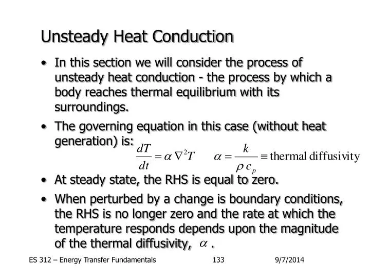
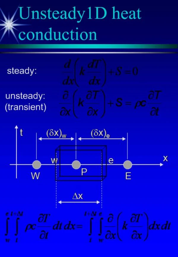
1. Unsteady Heat Conduction • In this section we will consider the process of unsteady heat conduction - the process by which a body reaches thermal equilibrium with its surroundings. • The governing equation in this case (without heat generation) is: • At steady state, the RHS is equal to zero. • When perturbed by a change is boundary conditions, the RHS is no longer zero and the rate at which the temperature responds depends upon the magnitude of the thermal diffusivity, . ES 312 – Energy Transfer Fundamentals

2. Ti h h T T x L -L Unsteady Heat Conduction (cont) • Consider the following case of a wall initial at equilibrium at T0, suddenly exposed to a cooling convective stream at T. • Let’s non-dimensionalize this problem by using the following definitions: • Where Lc is a characteristic length (probably L), and tc is a characteristic time period. AE 301 Aerodynamics I

3. Unsteady Heat Conduction (cont) • Using these definitions, the governing equation may be re-written as: • The group of terms, (tc/Lc2), that is itself non-dimensional and is called the Fourier number, Fo. • The Fourier number is a useful indicator of how a body has responded: • A low value of Fo indicates that the body has not responded to changes yet except possibly near the boundaries. • A high value of Fo indicates that the body has had large changes in T and may in fact be near reaching a new equilibrium. AE 301 Aerodynamics I

4. Ti h h T T x L -L Unsteady Heat Conduction (cont) • The boundary condition (x = ±L) for this case is: • Or after non-dimensionalizing: • This introduces a new non-dimensional term, hLc/k, called the Biot number, Bi. • Another way to write Bi is: AE 301 Aerodynamics I

5. Unsteady Heat Conduction (cont) • Thus, Bi is the ratio of conduction to convection resistance. As a result: • A low value of Bi corresponds to a body with little internal temperature variation, but a large temperature jump at the surface (like copper). • A high value of Bi corresponds to a body with surface temperatures near the fluid temperature, but large internal temperature variations. • As a result of this non-dimensional analysis we can write that: • In the solutions that follow, we will see this functionality appear repeatedly. AE 301 Aerodynamics I

6. Unsteady Heat Conduction (cont) • A couple of final notes about our new factors of Fo and Bi. • For cases other than this simple planar wall, we define the characteristic length as the volume of the body divided by the convective surface area, As: • The Fourier number is usually written in terms of the time itself rather than a characteristic time. Thus: AE 301 Aerodynamics I

7. Lumped Heat Capacity • The first case we will consider is where Bi << 1. • In this case, the internal temperature variations are negligible and the body can be considered at a single temperature, T(t). • In this case, the energy entering the body through convection increases it’s energy (and T) by: • Defining , gives the governing equation: AE 301 Aerodynamics I

8. Lumped Heat Capacity (cont) • This equation and boundary condition are satisfied by: • Use this equation when ever heating a highly conductive material, a very small (thin) body, or where the convective cooling rate is very, very small. • Note: The Fourier number doesn’t appear in this eqn. Since the body is always in quasi-equilibrium internally. The rate process occurs on the surface, not the interior! AE 301 Aerodynamics I

9. Semi-Infinite Solids • The next approximate case to consider is the situation of a semi-infinite solid, as shown: • This case is also that of a finite width solid at very small values of Fo (time) such that only the region near the convection boundary has had time to respond. • Thus, the interior temperature is still at the initial value, Ti. Ti h k T x AE 301 Aerodynamics I

10. Semi-Infinite Solids (cont) • The governing eqn. in this situation is: • However, a simplified equation can be obtained by assuming similarity. I.e. that solutions for all t and x may be represented by functions of a single parameter given by: • Since: the governing eqn can be rewritten as: AE 301 Aerodynamics I

11. Semi-Infinite Solids (cont) • The governing eqn. in this situation is: • This ODE occurs fairly regularly and has known solutions. • For the most general boundary condition at x=0 where: • the solution is: AE 301 Aerodynamics I

12. Semi-Infinite Solids (cont) • Where the complimentary error function, erfc, is: • Tabulations of the error function are given in Appendix A. However, the results are also plotted parametrically in Figure 4-5, pg 140. • The curves in this figure are represented as: • Do you see the Bi and Fo numbers buried in this functionality? AE 301 Aerodynamics I

13. Semi-Infinite Solids (cont) • A simpler solution exists for the case where convection is very high and you can assume the surface temperature is equal to the fluid temp. • For this case, the initial condition and boundary condition at x=0 is: • the solution is: • A plot of these solutions if given on page 137 as Figure 4-4. AE 301 Aerodynamics I

14. Finite Thickness Solids • Finally, consider the more generalized case of a solid with finite dimensions and cooled equally on all sides. • The book gives analytic solutions for these cases when T(x,0) = Ti. • However, these solutions have also been presented graphically in Appendix C for plane walls, cylinders, and spheres. h h T T x L -L r ro h T AE 301 Aerodynamics I

15. Finite Thickness Solids (cont) • The graphs in section 4-4 (Fig. 4-7 to 4-16) actually come in three types: the time variation of the center temperature, the spatial variation within the body, and the total heat lost (gained). • The first plot, center temperature is in the form: • As Fo 0, this function goes to 1.0 indicating no change in the center temperature. • Thus, for Fo < 0.2, these charts are inaccurate and the semi-infinite solid method should be used. AE 301 Aerodynamics I

16. Finite Thickness Solids (cont) • The spatial variation is shown in a chart of: • From these we see that the spatial variation is very small for Bi < .1. For these cases, the lumped heat capacity method would work just as well. • The heat transfer charts show the variation in the current heat lost versus the final heat lost: AE 301 Aerodynamics I

17. 2H 2W y z 2L x Multi-Dimensional Effects • The previous method for slabs only accounted for a finite width in one dimension. Let’s extend this idea. • If we consider a generalized 3-D box, the governing eqn is: • Assume that separation of variables (in space) applies such that the solution will be: AE 301 Aerodynamics I

18. Multi-Dimensional Effects (cont) • The solution for each component is that for a finite slab in that direction, I.e: • The solution for each spatial axis is found from the Heisler charts on pages 142-150, and the combined 3-D solution from the previous equation. AE 301 Aerodynamics I

19. x r Multi-Dimensional Effects (cont) • Another similar problem is that of a cylinder of finite length. • This problem is 2-dimensional in r and x, such that: • And, with separation of the spatial variables, the solution will be in the form: 2L 2rO AE 301 Aerodynamics I

20. Multi-Dimensional Effects (cont) • The solution for each component is that for a finite slab in that direction, I.e: • As before, the solution in both spatial directions (x and r) are found and combined to obtained the 2-D solution. • Can you see how to also get 2-D solutions for something like a very long rectangular rod? AE 301 Aerodynamics I