Download
1 / 19
190 likes | 199 Views
This article explains and analyzes the Quicksort algorithm, including the steps involved in partitioning an array and the best and worst case scenarios. It also explores alternative analysis methods and possible tweaks to improve the performance of Quicksort.

E N D
Quicksort http://math.hws.edu/eck/jsdemo/sortlab.html
Quicksort I • To sort a[left...right]: 1.if left < right: 1.1.Partition a[left...right] such that: all a[left...p-1] are less than a[p], and all a[p+1...right] are >= a[p] 1.2.Quicksort a[left...p-1] 1.3.Quicksort a[p+1...right] 2.Terminate Source: David Matuszek
A key step in the Quicksort algorithm is partitioning the array We choose some (any) number p in the array to use as a pivot We partition the array into three parts: p p numbers greater than or equal top numbers less thanp Partitioning (Quicksort II)
Partitioning II • Choose an array value (say, the first) to use as the pivot • Starting from the left end, find the first element that is greater than or equal to the pivot • Searching backward from the right end, find the first element that is less than the pivot • Interchange (swap) these two elements • Repeat, searching from where we left off, until done
Partitioning • To partition a[left...right]: • p = a[left]; l = left + 1; r = right; 2.while l < r, do 2.1.while l < right && a[l] < p { l = l + 1; } 2.2.while r > left && a[r] >= p { r = r – 1;} 2.3.if l < r { swap a[l] and a[r] } 3.a[left] = a[r]; a[r] = p; 4. Terminate
Example of partitioning • choose pivot: 4 3 6 9 2 4 3 1 2 1 8 9 3 5 6 • search: 436 9 2 4 3 1 2 1 8 9 35 6 • swap: 433 9 2 4 3 1 2 1 8 9 65 6 • search: 43 39 2 4 3 1 2 18 9 65 6 • swap: 43 31 2 4 3 1 2 98 9 65 6 • search: 43 31 24 3 1 298 9 65 6 • swap: 43 31 22 3 1 498 9 65 6 • search: 43 31 22 31498 9 65 6 (left > right) • swap with pivot: 13 31 22 34498 9 65 6
Analysis of quicksort—best case • Suppose each partition operation divides the array almost exactly in half • Then the depth of the recursion is log2n • because that’s how many times we can halve n • However, there are many recursions at each level! • How can we figure this out? • We note that • Each partition is linear over its subarray • All the partitions at one level cover the whole array
Best case II • We cut the array size in half each time • So the depth of the recursion is log2n • At each level of the recursion, all the partitions at that level do work that is linear in n • O(log2n) * O(n) = O(n log2n) • What about the worst case?
Worst case • In the worst case, partitioning always divides the size n array into these three parts: • A length one part, containing the pivot itself • A length zero part, and • A length n-1 part, containing everything else • We don’t recur on the zero-length part • Recurring on the length n-1 part requires (in the worst case) recurring to depth n-1
Worst case for quicksort • In the worst case, recursion may be O(n) levels deep (for an array of size n). • But the partitioning work done at each level is still O(n). • O(n) * O(n) = O(n2) • So worst case for Quicksort is O(n2) • When does this happen? • When the array is sorted to begin with!
Alternative Analysis Methods • See Weiss sections 7.7.5
Typical case for quicksort • If the array is sorted to begin with, Quicksort is terrible: O(n2) • It is possible to construct other bad cases • However, Quicksort is usuallyO(n log2n) • The constants are so good that Quicksort is the fastest general algorithm known • Most real-world sorting is done by Quicksort
Tweaking Quicksort • Almost anything you can try to “improve” Quicksort will actually slow it down • One good tweak is to switch to a different sorting method when the subarrays get small (say, 10 or 12) • Quicksort has too much overhead for small array sizes • For large arrays, it might be a good idea to check beforehand if the array is already sorted • But there is a better tweak than this
Picking a better pivot • Before, we picked the first element of the subarray to use as a pivot • If the array is already sorted, this results in O(n2) behavior • It’s no better if we pick the last element • Note that an array of identical elements is already sorted! • What if we pick a random pivot? (analyzed by Weiss, Sec. 7.7.5) • We could do an optimal quicksort (guaranteed O(n log n)) if we always picked a pivot value that exactly cuts the array in half • Such a value is called a median: half of the values in the array are larger, half are smaller • The easiest way to find the median is to sort the array and pick the value in the middle (!)
Median of three • Obviously, it doesn’t make sense to sort the array in order to find the median to use as a pivot • Instead, compare just three elements of our (sub)array—the first, the last, and the middle • Take the median (middle value) of these three as pivot • It’s possible (but not easy) to construct cases which will make this technique O(n2) • Suppose we rearrange (sort) these three numbers so that the smallest is in the first position, the largest in the last position, and the other in the middle • This lets us simplify and speed up the partition loop
Here’s the heart of the partition method: Because of the way we chose the pivot, we know that a[leftEnd] <= pivot <= a[rightEnd] Therefore a[l] < p will happen before l < right Likewise, a[r] >= p will happen before r > left Therefore the tests l < right and r > left can be omitted Simplifying the inner loop while (l < r) { while (l < right&& a[l] < p) l++; while (r > left&& a[r] >= p) r--; if (l < r) { int temp = a[l]; a[l] = a[r]; a[r] = temp; } }
Final comments • Weiss’s code shows some additional optimizations on pp. 246-247. • Weiss chooses to stop both searches on equality to pivot. This design decision is debatable. • Quicksort is the fastest known general sorting algorithm, on average. • For optimum speed, the pivot must be chosen carefully. • “Median of three” is a good technique for choosing the pivot. • There will be some cases where Quicksort runs in O(n2) time.