Download
1 / 56
760 likes | 1.58k Views
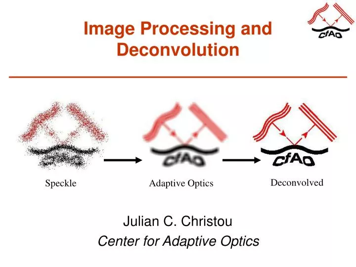
Image Processing and Deconvolution. Julian C. Christou Center for Adaptive Optics. Deconvolved. Speckle. Adaptive Optics. Outline. Introductory Mathematics Image Formation & Fourier Optics Deconvolution Schemes Linear – optimal filtering Non-Linear Conjugate Gradient Minimization

E N D
Image Processing andDeconvolution Julian C. Christou Center for Adaptive Optics Deconvolved Speckle Adaptive Optics
Outline • Introductory Mathematics • Image Formation & Fourier Optics • Deconvolution Schemes • Linear – optimal filtering • Non-Linear • Conjugate Gradient Minimization • - steepest descent search a la least squares • Lucy Richardson (LR) – Maximum Likelihood • Maximum a posteriori (MAP) • Regularization schemes • Other PSF calibration techniques • Quantitative Measurements
Why Deconvolution? • Better looking image • Improved identification • Reduces overlap of image structure to more easily identify features in the image (needs high SNR) • PSF calibration • Removes artifacts in the image due to the point spread function (PSF) of the system, i.e. extended halos, lumpy Airy rings etc. • Higher resolution • In specific cases depending upon algorithms and SNR • Better Quantitative Analysis
Image Formation • Image Formation is a convolution procedure for PSF invariance and incoherent imaging. • Convolution is a superposition integral, i.e. where i(r) – measured image p(r) – point spread function (impulse response function) o(r) – object distribution * - Convolution operator
Nomenclature In this presentation, the following symbols are used: g(r) – measured image h(r) – point spread function (impulse response function) f(r) – object distribution * - Convolution operator Relatively standardized nomenclature in the field.
Inverse Problems • The problem of reconstructing the original target falls into a class of Mathematics known as Inverse Problems which has its own Journal. References in diverse publications such as SPIEProceedings & IEEE Journals. • Multidisciplinary Field with many applications: • Applied Mathematics • - Matrix Inversion (SIAM) • Image and Signal Processing • - Medical Imaging (JOSA, Opt.Comm., Opt Let.) • - Astronomical Imaging (A.J., Ap.J., P.A.S.P., A.&A.) • OSA Topical Meetings on Signal Recovery & Synthesis
Fourier Transform Theorems • Autocorrelation Theorem • Convolution Theorem
Image Formation & Fourier Optics • Fraunhofer diffraction theory (far field): • The observed field distribution (complex wave in the focal plane) u(r) is approximated as the Fourier transform of the aperture distribution (complex wave at the pupil) P(r'). P(r') The point spread function (impulse response) is the square amplitude of the Fourier Transform of a plane wave sampled by the finite aperture, i.e. h(r) = |u(r)|2 = |FT{P(r')}|2 The power spectral density of the complex field at the pupil. h(r) • J. Goodman “Introduction to Fourier Optics”
MTF Normalized Spatial Frequency The Transfer Function • The Optical Transfer Function (OTF) is the spatial frequency response of the optical system. • The Modulation Transfer Function (MTF) is the modulus of the OTF and is the Fourier transform of the PSF.fc = /D From the autocorrelation theorem the MTF is the autocorrelation of the complex wavefront at the pupil.
The Fourier Domain Binary Stars Fourier Modulus Two delta functions produce a set of “fringes”, the frequency of which is inversely proportional to the separation and which are oriented along the separation vector. The “visibility” of the fringes corresponds to the intensity differences. How?
The Fourier Domain Gaussian Fourier Modulus (also Gaussian) These Fourier modulus of a Gaussian produces another Gaussian. A large object comprised of low spatial frequencies produces a compact Fourier modulus and a smaller object with higher spatial frequencies produces a larger Fourier modulus.
Fourier Relationships • Resolution of an aperture of size D is radians • Diffraction limit of an aperture of size D is cycles/radian • - resolution depends on wavelength and aperture • Large spatial structures correspond to low-spatial frequencies • Small spatial structures correspond to high-spatial frequencies
Image Formation - Convolution • Shift invariant imaging equation (Image and Fourier Domains) • Image Domain: • Fourier Domain: • g(r) - Measurement • f(r) - Object • h(r) - blur (point spread function) • g(r) - Noise contamination • Fourier Transform FT{g(r)} = G(f) etc. • * - convolution
Deconvolution The convolution equation is inverted. • Given the measurement g(r) and the PSF h(r) the object f(r) is computed. • e.g. • and inverse Fourier transform to obtain f(r). • Problem: • The PSF and the measurement are both band-limited due to the finite size of the aperture. • The object/target is not.
Images & Fourier Components ModulusPhase measurement PSF Left: Fourier amplitudes (ratio) Right: Fourier phases (difference) for the object. note circle = band-limit
Deconvolution via Linear Inversion Inverse Filtering:F(f) is a bandpass-limited attenuating filter, e.g. a chat function where H(f) = 0 for f > fc. Wiener Filtering: A noise-dependent filter -
Deconvolution via Linear Inversionwith a Wiener Filter - Example measurement PSF reconstruction Note the negativity in the reconstruction– not physical
Deconvolution Iterative non-linear techniques • Radio Astronomers, because of working with amplitude and phase signals, have far more experience with image/signal processing. • - Maximum Entropy Method • - CLEAN • Deconvolution (for visible astronomy) • HST - The Restoration of HST Images & Spectra, ed. R.J.Hanisch & R.L.White, STScI, 1993 • - Richardson-Lucy • - Pixon - Bayesian image reconstruction • - “Blind/Myopic” Deconvolution – poorly determined or unknown PSFs • - Maximum a posteriori • - Iterative Least Squares
A Simple Iterative Deconvolution Algorithm • Error Metric Minimization – object estimate & PSF convolve • to measurement • Strict positivity constraint • reparameterize the variable • Conjugate Gradient Search (least squares fitting) requires the first-order derivatives w.r.t. the variable, e.g. E /i • Equivalent to maximum-likelihood (the most probable solution) for Gaussian statistics • Permits “super-resolution”
Bayes Theorem on Conditional Probability P(A|B) P(B) = P(B|A) P(A) P – Probabilities A & B – Outcomes of random experiments P(A|B) - Probability of A given that B has occurred For Imaging: P(B|A) - Probability of measuring image B given that the object is A Fitting a probability model to a set of data and summarizing the result by a probability distribution on the model parameters and observed quantities.
Bayes Theorem on Conditional Probability • Setting up a full probability model – a joint probability distribution for all observable and unobservable quantities in a problem, • Conditioning on observed data: calculating and interpreting the appropriate posterior distribution – the conditional probability distribution of the unobserved quantities. • Evaluating the fit of the model. How good is the model?
Lucy-Richardson Algorithm Discrete Convolution where for all j From Bayes theorem P(gi|fj) = hij and the object distribution can be expressed iteratively as so that the LR kernel approaches unity as the iterations progress Richardson, W.H., “Bayesian-Based Iterative Method of Image Restoration”, J. Opt. Soc. Am., 62, 55, (1972). Lucy, L.B., “An iterative technique for the rectification of observed distributions”, Astron. J., 79, 745, (1974).
Richardson-Lucy ApplicationSimulated Multiple Star measurement PSF reconstruction Note – super-resolved result and identification of a 4th component Super-resolution means recovery of spatial frequency information beyond the cut-off frequency of the measurement system.
SNR = 2500 SNR = 250 SNR = 25 Truth 2000 iterations 200 iterations 26 iterations Diffraction limited PSF Richardson-Lucy ApplicationSimulated Galaxy All images on a logarithmic scale LR works best for high SNR
26 iterations 200 iterations 500 iterations 1000 iterations 2000 iterations 5000 iterations Richardson-Lucy ApplicationNoise Amplification • Maximum-likelihood techniques suffer from noise amplification • Problem is knowing when to stop • SNR = 250 Measurement diffraction limited All images on a logarithmic scale
Richardson-Lucy ApplicationNoise Amplification • For small iterations RL produces spatial frequency components not strongly filtered by the OTF, i.e. the low spatial frequencies. • Spatial frequencies which are strongly filtered by the OTF will take many iterations to reconstruct (the algorithm is relatively unresponsive), i.e. the high spatial frequencies. • In the presence of noise, the implication is that after many iterations the differences are small and are likely to be due to noise amplification. • This is a problem with any of these types of algorithms which use maximum-likelihood approaches including error metric minimization schemes.
No smoothing 0.5 pixels 1 pixels Diffraction limited Richardson-Lucy ApplicationRegularization Schemes • Sophisticated and silly! • Why not smooth the result? – a low-pass filtering! SNR = 250 – 5000 iterations • What is the reliability of the high SNR region? • Is it oversmoothed or undersmoothed?
Maximum a posteriori (MAP) Regularized Maximum-likelihood The posterior probability comes from Bayesian approaches, i.e. the probability of f being the object given the measurement g is: where P(g|f) = and P(f) is now the prior probability distribution (prior)
Maximum a posteriori (MAP) • Poisson maximum a posteriori - Hunt & Semintilli • denotes convolution • denotes correlation • Positivity assured by exponential • Non-linearity permits super-resolution, i.e. recovery of spatial frequencies for f > fc
Other Regularization Schemes • Physical Constraints • Object positivity • Object support (finite size of the object, e.g. a star is a point) • Object model • Parametric • texture • Noise modeling • The imaging process
Regularization Schemes • Reparameterization of the object with a smoothing kernel – (sieve function or low-pass filter). • Truncated iterations stop convergence when the error-metric reaches the noise-limit, , such that
Object Prior Information Prior information about the target can be used to modify the general algorithm. • Multiple point source field – N sources Solve for three parameters per component: amplitude Aj location rj
Object Prior Information Planetary/hard-edged objects (avoids ringing) (Conan et al, 2000) Use of the finite-difference gradients f(r) to generate an extra error term which preserves hard edges in f(r). & are adjustable parameters.
Object Prior Regularization - Texture Generalized Gauss-Markov Random Field Model (Jeffs) a.k.a. Object “texture” – local gradient bi,j - neighbourhood influence parameter p - shape parameter
Object Prior Regularization Generalized Gauss-Markov Random Field Model truth raw over under
The Imaging Process Model the preprocessing in the imaging process • Light from target to the detector • Through optical path – PSF • Detector • Gain – (flat field) a(r) • Dark current – (darks) d(r) • Background – (sky) b(r) • Hot and dead pixels – included in a(r) • Noise • Most algorithms work with “corrected” data • Forward model the estimate to compare with the measurement truth raw
PSF Calibration:Variations on a Theme • Poor or no PSF estimate – Myopic/Blind Deconvolution • Astronomical imaging typically measures a point source reference • sequence with the target. • - Long exposure – standard deconvolution techniques • - Short exposure – speckle techniques – e.g. power spectrum & bispectrum • Deconvolution from wavefront sensing (DWFS) • Use a simultaneously obtained wavefront to deconvolve the • focal-plane data frame-by-frame. PSF generated from • wavefront. • Phase Diversity • Two channel imaging typically in & out of focus. Permits • restoration of target and PSF simultaneously. No PSF • measurement needed.
Blind Deconvolution contamination Measurement unknown object unknown or poorly known PSF Need to solve for both object & PSF “It’s not only impossible, it’s hopelessly impossible”
Blind Deconvolution – Key Papers Ayers & Dainty, “Iterative blind deconvolution and its applications” , Opt. Lett. 13 , 547-549, 1988. Holmes , “Blind deconvolution of speckle images quantum-limited incoherent imagery: maximum-likelihood approach” , J. Opt. Soc. Am. A, 9 , 1052-106, 1992. Lane , “Blind deconvolution of speckle images” , J. Opt. Soc. Am. A, 9 , 1508-1514, 1992 . Jefferies & Christou, “Restoration of astronomical images by iterative blind deconvolution” , Astrophys. J.415, 862-874, 1993. Schultz , “Multiframe blind deconvolution of astronomical images” , J. Opt. Soc. Am. A, 10 , 1064-1073, 1993. Thiebaut & Conan, “Strict a priori constraints for maximum-likelihood blind deconvolution” , J. Opt. Soc. Am. A, 12 , 485-492, 1995. Conan et al., “Myopic deconvolution of adaptive optics images by use of object and point-spread function power spectra”, Appl. Opt., 37, 4614-4622, 1998 .
Multiple Frame Blind Deconvolution m independent observations of the same object. The problem reduces from 1 measurement & 2 unknowns to m measurements & m+1 unknowns
Physical Constraints • “Blind” deconvolution solves for both object & PSF simultaneously. • Ill-posed inverse problem. • Under – determined: 1 measurement, 2 unknowns • Uses Physical Constraints. • f(r) & h(r) are positive, real & have finite support. • Finite support reduces # of variables (symmetry breaking) • h(r) is band-limited – symmetry breaking • a priori information - further symmetry breaking (a * b = b * a) • Prior knowledge • PSF knowledge: band-limit, known pupil, statistical derived PSF • Object & PSF parameterization: multiple star systems • Noise statistics
Io in Eclipse (Marchis et al.) Two Different BD Algorithms Keck observations to identify hot-spots. K-Band 19 with IDAC 17 with MISTRAL L-Band 23 with IDAC 12 with MISTRAL
Solar Imaging • Rimmele, Marino & Christou • AO Solar Images from National Solar Observatory low-order system. Sunspot Feature – improves contrast, enhances detail showing magnetic field structure
IRS 10 IRS 5 IRS 10 IRS 1W IRS 21 IRS 1W IRS 21 Extended Sources near the Galactic Center Tanner et al. Deconvolution permits easier determination of extended sources of astrophysical interest
Deconvolution from Wavefront Sensing Multiframe deconvolution with a “known” PSF. The estimate of the Fourier components of the target for a series of short-exposure observations is (Primot et al.) (also see speckle holography) where | H`(f) |2 = H`(f) H`(f)* and H`(f) is the PSF estimate obtained from the measured wavefront, i.e. the autocorrelation of the complex wavefront at the pupil. F`(f) = F(f) when H`(f) = H(f) Noise sensitive transfer function. Requires good SNR modeling. Primot et al. “Deconvolution from wavefront sensing: a new technique for compensating turbulence-degraded images” , J. Opt. Soc. Am. A, 7, 1598-1608, 1990.
Phase Diversity Measurement of the object in two different channels. No separate PSF measurement. Two measurements – 3 unknowns – f(r), h1(r), h2(r) but h1(r) & h2(r) are related by a known diversity, e.g. defocus. Hence 2 unknownsf(r), h1(r)
Phase Diversity • Phase Diversity restores both the target and the complex wavefront phases at the pupil. • Solve for the wavefront phases which represent the unknowns for the PSFs • The phases can be represented as either • - zonal (pixel-by-pixel) • - modal (e.g. Zernike modes) – fewer unknowns • The object spectrum can be written in terms of the wavefront phases, i.e. • Recent work suggests that solving for the complex wavefront, i.e. modeling scintillation improved PD performance for both object and phase recovery.
Photometric Quality in Crowded fields Busko, 1993 HST Tests “Should stellar photometry be done on restored or unrestored images?”