CHAPTER OUTLINE

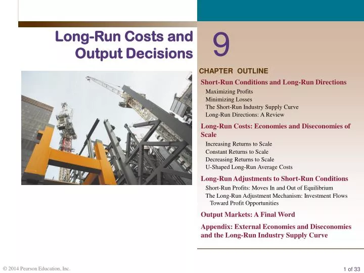
1. 9 Long-Run Costs and Output Decisions CHAPTER OUTLINE Short-Run Conditions and Long-Run Directions Maximizing Profits Minimizing Losses The Short-Run Industry Supply Curve Long-Run Directions: A Review Long-Run Costs: Economies and Diseconomies of Scale Increasing Returns to Scale Constant Returns to Scale Decreasing Returns to Scale U-Shaped Long-Run Average Costs Long-Run Adjustments to Short-Run Conditions Short-Run Profits: Moves In and Out of Equilibrium The Long-Run Adjustment Mechanism: Investment Flows Toward Profit Opportunities Output Markets: A Final Word Appendix: External Economies and Diseconomies and the Long-Run Industry Supply Curve

2. We begin our discussion of the long run by looking at firms in three short-run circumstances: • Firms that earn economic profits. • Firms that suffer economic losses but continue to operate to reduce or minimize those losses. • Firms that decide to shut down and bear losses just equal to fixed costs.

3. Short-Run Conditions and Long-Run Directions breaking evenThe situation in which a firm is earning exactly a normal rate of return. Maximizing Profits Example: The Blue Velvet Car Wash: earning a (+) economic profit

4. 1 Normal rate of return = 0 Economic Profit Economists include all opportunity costs when analyzing a firm, whereas accountants measure only explicit costs. Therefore, economic profit is smaller than accounting profit

5. Graphic Presentation  FIGURE 9.1Firm Earning a Positive Profit in the Short Run • produce up to the point where P* = MC. • At q* = 800, total revenue is $5 × 800 = $4,000, total cost is $4.50 × 800 = $3,600, and profit = $4,000  $3,600 = $400. Because average total cost is derived by dividing total cost by q, we can get back to total cost by multiplying average total cost by q. TC = ATC × q. and so

6. Minimizing Losses ■ If total revenue exceeds total variable cost, the excess revenue can be used to offset fixed costs and reduce losses, and it will pay the firm to keep operating. (so produce if Pmkt> AVCmin) ■ If total revenue is smaller than total variable cost, the firm that operates will suffer losses in excess of fixed costs. In this case, the firm can minimize its losses by shutting down. Pmkt<AVCmin Producing at a Loss to Offset Fixed Costs shutdown pointThe lowest point on the average variable cost curve. When price falls below the minimum point on AVC, total revenue is insufficient to cover variable costs and the firm will shut down and bear losses equal to fixed costs.

7.  FIGURE 9.2Short-Run Supply Curve of a Perfectly Competitive Firm At prices below average variable cost, it pays a firm to shut down rather than continue operating. Thus, the short-run supply curve of a competitive firm is the part of its marginal cost curve that lies above its average variable cost curve.

8. Long-Run Costs: Economies and Diseconomies of Scale • increasing returns to scale, or economies of scaleAn increase in a firm’s scale of production leads to lower costs per unit produced. • large fixed costs – hydroelectric dams • constant returns to scaleAn increase in a firm’s scale of production has no effect on costs per unit produced. Costs per unit remain the same as production expands • Cellular services: expand with antennas • decreasing returns to scale, or diseconomies of scaleAn increase in a firm’s scale of production leads to higher costs per unit produced. • Very little fixed costs, or • Fixed factor – “entrepreneurial ability” - there’s only 1 Steve Jobs

9. Increasing Returns to Scale The Sources of Economies of Scale • Economics of scale have come from advantages of larger firm size rather than gains from plant size. • Large Fixed Costs • Hydroelectric dams • Grand Coulee - $450M; produces 6809MW – 6,809,000 kW • Average house – 1.5 kW • Verizon/GTE consolidation • Prior to consolidation • 8 separate companies each with own forecasting, billing departments and management (total forecast = 400) • Consolidation • 1 corporate headquarters: (forecasters = 100); 1 billing department; around the clock repair/trouble service (time-shifting)

10. 6 Average Total Cost Average total cost in the short and long runs ATC in short run with medium factory ATC in long run ATC in short run with large factory ATC in short run with small factory $12,000 Constant returns to scale 10,000 Diseconomies of scale Economies of scale 0 Quantity of Cars per Day 1,000 1,200 Because fixed costs are variable in the long run, the average-total-cost curve in the short run differs from the average-total-cost curve in the long run.

11. Graphic Presentation long-run average cost curve (LRAC)The “envelope” of a series of short-run cost curves. minimum efficient scale (MES)The smallest size at which the long-run average cost curve is at its minimum.  FIGURE 9.4A Firm Exhibiting Economies of Scale In the LR- all costs are variable – you can choose any scale. In the SR – after you choose a scale (e.g., Scale 2) you are then on that SRAC/SRMC curve until you can change the scale

12. E C O N O M I C S I N P R A C T I C E Economies of Scale in Solar The process of producing solar panels is subject to scale economies, so that as the use of solar panels increases, the long-run average cost of producing them is likely to fall. It is an open question about just how low costs of solar energy might ever be. In new technologies it is not easy to figure out just how large scale economies might be, given that firms have little experience with expanding firm size, and doing so carries some risks. • THINKING PRACTICALLY • How does the price of oil affect a firm’s willingness to experiment with large scale solar energy production?

13. Constant Returns to Scale Technically, the term constant returns means that the quantitative relationship between input and output stays constant, or the same, when output is increased. Constant returns to scale mean that the firm’s long-run average cost curve remains flat. Decreasing Returns to Scale When average cost increases with scale of production, a firm faces decreasing returns to scale, or diseconomies of scale.

14. U-Shaped Long-Run Average Costs  FIGURE 9.5A Firm Exhibiting Economies and Diseconomies of Scale Economies of scale push this firm’s average costs down to q*. Beyond q*, the firm experiences diseconomies of scale; q* is the level of production at lowest average cost, using optimal scale. optimal scale of plantThe scale of plant that minimizes average cost given expected Demand

15. Long-Run Adjustments to Short-Run Conditions Short-Run Profits: Moves In and Out of Equilibrium  FIGURE 9.6Equilibrium for an Industry with U-shaped Cost Curves The individual firm on the right is producing 2,000 units, and so we also know that the industry consists of 100 firms. All firms are identical, and all are producing at the uniquely best output level of 2,000 units.

16.  FIGURE 9.7Industry Response to an Increase in Demand

17.  FIGURE 9.8New Equilibrium with Higher Demand

18. In equilibrium, each firm has SRMC = SRAC = LRAC Firms make no excess profits so that P = SRMC = SRAC = LRAC and there are enough firms so that supply equals demand.

19. E C O N O M I C S I N P R A C T I C E The Fortunes of the Auto Industry In 2010 the U.S. government was a “reluctant shareholder” in General Motors to help the firm move out of the bankruptcy that it entered in 2009. By 2010, General Motors had returned to profitability. The demand for autos shifted right as the recession eased, and this allowed GM to raise prices and sell more vehicles. Improved sales also helped on the cost side. The auto industry exhibits large economies of scale due in part to the large capital investment of the assembly lines. In the 2008–2009 recession, the auto industry found itself with excess capacity, and the per-unit costs of cars rocketed up. By using more of its capacity, average costs fell, making for better profitability. • THINKING PRACTICALLY • How did this change the long-run AC curve?

20. The Long-Run Adjustment Mechanism: Investment Flows Toward Profit Opportunities The entry and exit of firms in response to profit opportunities usually involve the financial capital market. In capital markets, people are constantly looking for profits. When firms in an industry do well, capital is likely to flow into that industry in a variety of forms. long-run competitive equilibriumWhen P = SRMC = SRAC = LRAC and profits are zero. Investment—in the form of new firms and expanding old firms—will over time tend to favor those industries in which profits are being made; and over time, industries in which firms are suffering losses will gradually contract from disinvestment.

21. E C O N O M I C S I N P R A C T I C E Why Are Hot Dogs So Expensive in Central Park? In New York, you need a license to operate a hot dog cart, and a license to operate in the park costs more. Since hot dogs are $0.50 more in the park, the added cost of a license each year must be roughly $0.50 per hot dog sold. In fact, in New York City, licenses to sell hot dogs in the park are auctioned off for many thousands of dollars, while licenses to operate in more remote parts of the city cost only about $1,000. • THINKING PRACTICALLY • Show on a graph how a higher-priced license increases hot dog prices. • Who is the woman in the coat?

22. Output Markets: A Final Word In the last four chapters, we have been building a model of a simple market system under the assumption of perfect competition. In our wine example, higher demand leads to higher prices, and wine producers find themselves earning positive profits. This increase in price and consequent rise in profits is the basic signal that leads to a reallocation of society’s resources. In the short run, wine producers are constrained by their current scales of operation. In the long run, however, we would expect to see resources flow in to compete for these profits. What starts as a shift in preferences thus ends up as a shift in resources. You have now seen what lies behind the demand curves and supply curves in competitive output markets. The next two chapters take up competitive input markets and complete the picture.

23. R E V I E W T E R M S A N D C O N C E P T S breaking even constant returns to scale decreasing returns to scale or diseconomies of scale increasing returns to scale or economies of scale long-run average cost curve (LRAC) long-run competitive equilibrium minimum efficient scale (MES) optimal scale of plant short-run industry supply curve shutdown point long-run competitive equilibrium, P = SRMC = SRAC = LRAC

24. CHAPTER 9 APPENDIX External Economies and Diseconomies and the Long-Run IndustrySupply Curve When long-run average costs decrease as a result of industry growth, we say that there are external economies. When average costs increase as a result of industry growth, we say that there are external diseconomies.

25. The Long-Run Industry Supply Curve long-run industry supply curve (LRIS) A curve that traces out price and total output over time as an industry expands. decreasing-cost industry An industry that realizes external economies—that is, average costs decrease as the industry grows. The long-run supply curve for such an industry has a negative slope. increasing-cost industry An industry that encounters external diseconomies—that is, average costs increase as the industry grows. The long-run supply curve for such an industry has a positive slope. constant-cost industry An industry that shows no economies or diseconomies of scale as the industry grows. Such industries have flat, or horizontal, long-run supply curves.

26.  FIGURE 9A.1A Decreasing-Cost Industry: External Economies In a decreasing-cost industry, average cost declines as the industry expands. As demand expands from D0 to D1, price rises from P0 to P1. As new firms enter and existing firms expand, supply shifts from S0 to S1, driving price down. If costs decline as a result of the expansion to LRAC2, the final price will be below P0 at P2. The long-run industry supply curve (LRIS) slopes downward in a decreasing-cost industry.

27.  FIGURE 9A.2An Increasing-Cost Industry: External Diseconomies In an increasing-cost industry, average cost increases as the industry expands. As demand shifts from D0 to D1, price rises from P0 to P1. As new firms enter and existing firms expand output, supply shifts from S0 to S1, driving price down. If long-run average costs rise, as a result, to LRAC2, the final price will be P2. The long-run industry supply curve (LRIS) slopes up in an increasing-cost industry.

28. constant-cost industry decreasing-cost industry external economies and diseconomies increasing-cost industry long-run industry supply curve (LRIS) A P P E N D I X R E V I E W T E R M S A N D C O N C E P T S