Download
1 / 29
290 likes | 463 Views
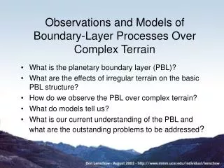
Observations and Models of Boundary-Layer Processes Over Complex Terrain. What is the planetary boundary layer (PBL)? What are the effects of irregular terrain on the basic PBL structure? How do we observe the PBL over complex terrain? What do models tell us?

E N D
Observations and Models of Boundary-Layer Processes Over Complex Terrain • What is the planetary boundary layer (PBL)? • What are the effects of irregular terrain on the basic PBL structure? • How do we observe the PBL over complex terrain? • What do models tell us? • What is our current understanding of the PBL and what are the outstanding problems to be addressed?
Overview of problems and possible future directions • Most theoretical, modeling and observational results are applicable to a horizontally homogeneous PBL and underlying surface. • Non-uniform surfaces predominate over land. • New tools are needed and are becoming available to address PBL structure over heterogeneous terrain.
Comparison of remote Doppler radial velocity statistics (30 m vertical resolution) from the Wyoming Cloud Radar with in situ measurements during DYCOMS-II obtained from 30 minute (180 km) circles. Variance Turbulence dissipation
daytime z = 40 m
Schematic of complex flows and effects on CO at forest-lake boundary with nocturnal stably-stratified flow
Even minimal terrain slope can affect e.g. surface wind direction in the stably-stratified PBL. Caughey et al., JAS, 1979 noted from the Minnesota experiment that surface wind rotation through the evening transition was affected by a terrain slope of 0.0014 (0.08°).
Vertical velocity at 8 levels on the 60 m CASES99 tower on the night of 18 Oct 1999. Strong turbulent mixing is associated with 3 different events: 1) a density current, 2) a solitary wave, and 3) an internal gravity wave. Vertical velocity is shifted by the amount given at the right of each time series. (From Sun, et al., BLM, 2003.)
Time-height cross- • sections of: • air temperature • specific humidity • wind speed • wind direction • vertical velocity • at 8 levels • relative variations • of CO at 5, 20, • and 40 m
FM-CW radar image between 1100 and 1200 UTC showing radar backscatter from refractivity fluctuations (moisture). (Univ. of Massachusetts S-band 11 cm FM-CW radar with 2.5 m resolution within a 3° beam.) From Sun et al., 50 m tower height time series of : (a) vertical velocity and air temperature (b) wind speed and direction
MAP-Riviera Project – summer-autumn 1999 – investigate boundary layer and hydrology, including turbulence exchange processes in one exemplary alpine valley (Weigel and Rotach, 2003).
Tower and Aircraft measurements Eco-Dimona HB 2335 (930 kg) Measurement of wind speed, temperature and moisture with temporal resolution of 10 Hz
How to determine zi ? • Temperature profiles often lack a clear inversion • Apply TKE-threshold criterium for boundary layer thickness: zi = where TKE < 0.4m2/s2
Main Reference Sources for these Lectures Belcher, S.E. and J.C.R. Hunt, 1998: Turbulent flow over hills and waves. Annu. Rev. Fluid Mech.. 30:507-538. Blumen, W., 1990: Atmospheric Processes Over Complex Terrain. American Meteorological Society, Boston, MA. Geiger, R., R.H. Aron and P. Todhunter, 1961: The Climate Near the Ground. Vieweg & Son, Braunschweig. Kaimal, J.C. and J.J. Finnigan, 1994: Atmospheric Boundary Layer Flows. Oxford Univ. Press, New York. Oke, T.R., 1987: Boundary Layer Climates. Routledge, New York. Venkatram, A. and J.C. Wyngaard, Eds.,1988: Lectures on Air Pollution Modeling. American Meteorological Society, Boston MA. Abstracts from the10th Conference on Mountain Meteorology, 17-21 June 2002, Park City, UT, American Meteorological Society, Boston. Suggestions for Further Reading