Download
1 / 47
490 likes | 935 Views
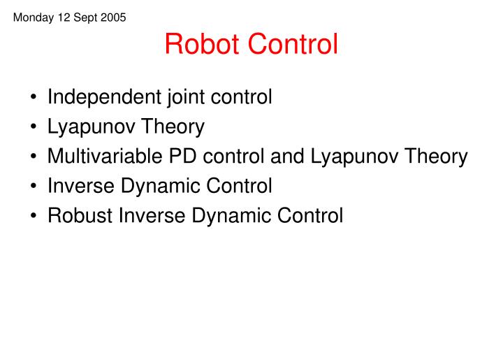
Monday 12 Sept 2005. Robot Control. Independent joint control Lyapunov Theory Multivariable PD control and Lyapunov Theory Inverse Dynamic Control Robust Inverse Dynamic Control. Feedforward Compensation – Independent Joint. +. +. -. Chain Rule:.

E N D
Monday 12 Sept 2005 Robot Control • Independent joint control • Lyapunov Theory • Multivariable PD control and Lyapunov Theory • Inverse Dynamic Control • Robust Inverse Dynamic Control
, equivalently the quadratic form, is said to be positive definite if and only if , will be positive definite if and only if the matrix P is positive definite matrix, that is, has all eigenvalues positive.
Theorem: The null solution of is asymptotically stable if there exists a Lyapunov function candidate V such that is negative definite along solution trajectories, that is,
LaSalle’s Theorem: Given the system suppose a Lyapunov function candidate V such that along solution trajectories Then the above system is asymptotically stable if does not vanish identically along any solution of the above system other than the null solution, that is, the system is asymptotically stable if the only solution of the system satisfying is the null solution.
Example: V-dot is zero when x2 is zero. When x2 is zero (in steady-state) then its rate of change also must be zero so x1 has to be identically zero from the second equation. So finally the rate of change of x1 should be zero from the first equation hence V is identically zero only along the equilibrium solution (0,0) of the system. Hence according to LaSalle’s Theorem the system is asymptotically stable.
Independent joint PD-control Scheme Simplify V-dot. Is this sign definite?
Theorem 6.3.1 (p. 143 of the textbook) Define the matrix Then is skew symmetric, that is, the components Proof: Since the inertia matrix D(q) is symmetric, it is not difficult to see that N is skew symmetric.
Independent joint PD-control Scheme • We neglect the gravity terms or add an extra term g(q) in the input u. • We choose KD such that KD +B is positive definite. • This makes V-dot negative semi-definite.
When V-dot is identically equal to zero then it implies that q-dot and q-double dot are both identically equal to zero. But this doesn’t imply that the error is zero, i.e., q-desired may not equal q. But from we see that when v-dot is zero we must have LaSalle’s Theorem then implies that the system is asymptotically stable. To account for the gravity torque we can either have the position gains Kp very large or modify the input expression as
Nominally linear system Trajectory planner Robust compensator Nonlinear interface Plant Inner loop Outer loop
Trajectory Interpolation Solve for (a,b,c,d,e).
//(1) trajectory planning //(2) simulation of inverse dynamic control of one link manipulator //I*theta-double dot+MgL*sin(theta) = u //10 Sept 2005 //Go to the directory where you keep this file and then to run it //exec('invdynpendulum.sce') clear t0 t1 t2 t I Ihat Mglhat k0 k1 dt abcde pos speed acc x1 x2 z m traj t0=0; t1=0.5; t2=1; I=5;Mgl=10;Ihat=5;Mglhat=5; k0=10;k1=10;dt=0.01; //theta=a+b*t+c*t^2+d*t^3+e*t^4 traj=[0;1;1;0;0];//position at t=t0, t=t1, t=t2; speed at t=t2; acceleration at t=t2 m=[1,t0,t0^2,t0^3,t0^4;1,t1,t1^2,t1^3,t1^4;1,t2,t2^2,t2^3,t2^4;0,1,2*t2,3*t2^2,4*t2^3;0,0,2,6*t2,12*t2^2]; abcde=inv(m)*traj; t=[0:dt:1]; pos=abcde'*[ones(size(t,1),size(t,2));t;t.*t;(t.*t).*t;(t.*t).*(t.*t)]; speed=abcde'*[zeros(size(t,1),size(t,2));ones(size(t,1),size(t,2));2*t;3*(t.*t);4*(t.*t).*t]; acc=abcde'*[zeros(size(t,1),size(t,2));zeros(size(t,1),size(t,2));... 2*ones(size(t,1),size(t,2));6*(t);12*t.*t]; x1(1)=pos(1); x2(1) = speed(1); z=[x1(1);x2(1)]; //initial conditions for k = 2:size(t,2), z(1)=z(1)+z(2)*dt; z(2)=z(2)+(-Mgl*sin(z(1))+Ihat*(acc(k)+k1*(speed(k)-z(2))+k0*(pos(k)-z(1)))+Mglhat*sin(z(1)))*(dt/I); x1(k)=z(1);x2(k)=z(2); end; f1=scf(1);clf(f1,'reset'); plot2d(t,pos,1);plot(t,x1,2); xgrid;xtitle('Theta', 'Time (s)','Angle (rad)');
desired desired k0=1, k1=2 I = 5, MgL = 10 k0=10, k1=10
We need to choose the control such that
This is not likely because of the zero elements of the upper left quarter of the matrix. This means we have to try another Lyapunov function candidate. Find
This should be possible. So choose the P matrix and K0 and K1 such that Q is negative definite.
//(1) trajectory planning //(2) simulation of inverse dynamic control of one link manipulator //I*theta-double dot+MgL*sin(theta) = u //10 Sept 2005 //Go to the directory where you keep this file and then to run it //exec('invdynpendulum.sce') clear t0 t1 t2 t I Ihat Mglhat k0 k1 dt abcde pos speed acc x1 x2 z m traj Q1 t0=0; t1=0.5; t2=1; I=5;Mgl=10;Ihat=7.5;Mglhat=7.5; k0=1;k1=2;dt=0.01; alpha=0.5;Mbar=0.2; phi=2.5;p11=1;p12=1;p21=11;p22=1; //theta=a+b*t+c*t^2+d*t^3+e*t^4 traj=[0;1;1;0;0];//position at t=t0, t=t1, t=t2; speed at t=t2; acceleration at t=t2 m=[1,t0,t0^2,t0^3,t0^4;1,t1,t1^2,t1^3,t1^4;1,t2,t2^2,t2^3,t2^4;0,1,2*t2,3*t2^2,4*t2^3;0,0,2,6*t2,12*t2^2]; abcde=inv(m)*traj; t=[0:dt:1]; pos=abcde'*[ones(size(t,1),size(t,2));t;t.*t;(t.*t).*t;(t.*t).*(t.*t)]; speed=abcde'*[zeros(size(t,1),size(t,2));ones(size(t,1),size(t,2));2*t;3*(t.*t);4*(t.*t).*t]; acc=abcde'*[zeros(size(t,1),size(t,2));zeros(size(t,1),size(t,2));... 2*ones(size(t,1),size(t,2));6*(t);12*t.*t]; Q1=max(acc);
x1(1)=pos(1); x2(1) = speed(1); z=[x1(1);x2(1)]; //initial conditions for k = 2:size(t,2), etheta=z(1)-pos(k); espeed=z(2)-speed(k); rho=(1/(1-alpha))*(alpha*Q1+alpha*sqrt(k0*k0+k1*k1)*sqrt(etheta*etheta+espeed*espeed)+Mbar*phi); if abs(z(2)+z(1)) > 0.0000000001 then delv=-rho*(etheta+espeed)/abs((etheta+espeed)); else delv=0; end; z(1)=z(1)+z(2)*dt; z(2)=z(2)+(-Mgl*sin(z(1))+Ihat*(acc(k)+k1*(speed(k)-z(2))+k0*(pos(k)-z(1))+delv)+Mglhat*sin(z(1)))*(dt/I); x1(k)=z(1);x2(k)=z(2); end; f1=scf(1);clf(f1,'reset'); plot2d(t,pos,1);plot(t,x1,2); xgrid;xtitle('Theta', 'Time (s)','Angle (rad)');
desired desired k0=1, k1=2 I = 5, MgL = 10