Download
1 / 20
630 likes | 4.08k Views
Lazy vs. Eager Learning. Lazy vs. eager learning Lazy learning (e.g., instance-based learning): Simply stores training data (or only minor processing) and waits until it is given a test tuple

E N D
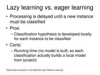
Lazy vs. Eager Learning • Lazy vs. eager learning • Lazy learning (e.g., instance-based learning): Simply stores training data (or only minor processing) and waits until it is given a test tuple • Eager learning (the above discussed methods): Given a set of training set, constructs a classification model before receiving new (e.g., test) data to classify • Lazy: less time in training but more time in predicting Data Mining: Concepts and Techniques
Lazy Learner: Instance-Based Methods • Instance-based learning: • Store training examples and delay the processing (“lazy evaluation”) until a new instance must be classified • Typical approaches • k-nearest neighbor approach • Instances represented as points in a Euclidean space. • Locally weighted regression • Constructs local approximation • Case-based reasoning • Uses symbolic representations and knowledge-based inference Data Mining: Concepts and Techniques
The k-Nearest Neighbor Algorithm • All instances correspond to points in the n-D space • The nearest neighbor are defined in terms of Euclidean distance, dist(X1, X2) • Target function could be discrete- or real- valued • For discrete-valued, k-NN returns the most common value among the k training examples nearest toxq • Vonoroi diagram: the decision surface induced by 1-NN for a typical set of training examples . _ _ _ . _ . + . + . _ + xq . _ + Data Mining: Concepts and Techniques
Discussion on the k-NN Algorithm • k-NN for real-valued prediction for a given unknown tuple • Returns the mean values of the k nearest neighbors • Distance-weighted nearest neighbor algorithm • Weight the contribution of each of the k neighbors according to their distance to the query xq • Give greater weight to closer neighbors • Robust to noisy data by averaging k-nearest neighbors • Curse of dimensionality: distance between neighbors could be dominated by irrelevant attributes • To overcome it, elimination of the least relevant attributes Data Mining: Concepts and Techniques
Genetic Algorithms (GA) • Genetic Algorithm: based on an analogy to biological evolution • An initial population is created consisting of randomly generated rules • Each rule is represented by a string of bits • E.g., if A1 and ¬A2 then C2 can be encoded as 100 • If an attribute has k > 2 values, k bits can be used • Based on the notion of survival of the fittest, a new population is formed to consist of the fittest rules and their offsprings • The fitness of a rule is represented by its classification accuracy on a set of training examples • Offsprings are generated by crossover and mutation • The process continues until a population P evolves when each rule in P satisfies a prespecified threshold • Slow but easily parallelizable Data Mining: Concepts and Techniques
Rough Set Approach • Rough sets are used to approximately or “roughly” define equivalent classes • A rough set for a given class C is approximated by two sets: a lower approximation (certain to be in C) and an upper approximation (cannot be described as not belonging to C) • Finding the minimal subsets (reducts) of attributes for feature reduction is NP-hard but a discernibility matrix (which stores the differences between attribute values for each pair of data tuples) is used to reduce the computation intensity Data Mining: Concepts and Techniques
Fuzzy Set Approaches • Fuzzy logic uses truth values between 0.0 and 1.0 to represent the degree of membership (such as using fuzzy membership graph) • Attribute values are converted to fuzzy values • e.g., income is mapped into the discrete categories {low, medium, high} with fuzzy values calculated • For a given new sample, more than one fuzzy value may apply • Each applicable rule contributes a vote for membership in the categories • Typically, the truth values for each predicted category are summed, and these sums are combined Data Mining: Concepts and Techniques
Classifier Accuracy Measures • Accuracy of a classifier M, acc(M): percentage of test set tuples that are correctly classified by the model M • Error rate (misclassification rate) of M = 1 – acc(M) • Given m classes, CMi,j, an entry in a confusion matrix, indicates # of tuples in class i that are labeled by the classifier as class j • Alternative accuracy measures (e.g., for cancer diagnosis) sensitivity = t-pos/pos /* true positive recognition rate */ specificity = t-neg/neg /* true negative recognition rate */ precision = t-pos/(t-pos + f-pos) accuracy = sensitivity * pos/(pos + neg) + specificity * neg/(pos + neg) • This model can also be used for cost-benefit analysis Data Mining: Concepts and Techniques
Evaluating the Accuracy of a Classifier • Holdout method • Given data is randomly partitioned into two independent sets • Training set (e.g., 2/3) for model construction • Test set (e.g., 1/3) for accuracy estimation • Cross-validation (k-fold, where k = 10 is most popular) • Randomly partition the data into kmutually exclusive subsets, each approximately equal size • At i-th iteration, use Di as test set and others as training set • Leave-one-out: k folds where k = # of tuples, for small sized data Data Mining: Concepts and Techniques
Evaluating the Accuracy of a Classifier or Predictor (II) • Bootstrap • Works well with small data sets • Samples the given training tuples uniformly with replacement • i.e., each time a tuple is selected, it is equally likely to be selected again and re-added to the training set • Several boostrap methods, and a common one is .632 boostrap • Suppose we are given a data set of d tuples. The data set is sampled d times, with replacement, resulting in a training set of d samples. The data tuples that did not make it into the training set end up forming the test set. About 63.2% of the original data will end up in the bootstrap, and the remaining 36.8% will form the test set (since (1 – 1/d)d ≈ e-1 = 0.368) • Repeat the sampling procedue k times, overall accuracy of the model: Data Mining: Concepts and Techniques
Ensemble Methods: Increasing the Accuracy • Ensemble methods • Use a combination of models to increase accuracy • Combine a series of k learned models, M1, M2, …, Mk, with the aim of creating an improved model M* • Popular ensemble methods • Bagging: averaging the prediction over a collection of classifiers • Boosting: weighted vote with a collection of classifiers Data Mining: Concepts and Techniques
Bagging: Boostrap Aggregation • Analogy: Diagnosis based on multiple doctors’ majority vote • Training • Given a set D of d tuples, at each iteration i, a training set Di of d tuples is sampled with replacement from D (i.e., boostrap) • A classifier model Mi is learned for each training set Di • Classification: classify an unknown sample X • Each classifier Mi returns its class prediction • The bagged classifier M* counts the votes and assigns the class with the most votes to X • Prediction: can be applied to the prediction of continuous values by taking the average value of each prediction for a given test tuple • Accuracy • Often significant better than a single classifier derived from D • For noise data: not considerably worse, more robust • Proved improved accuracy in prediction Data Mining: Concepts and Techniques
Boosting • Analogy: Consult several doctors, based on a combination of weighted diagnoses—weight assigned based on the previous diagnosis accuracy • How boosting works? • Weights are assigned to each training tuple • A series of k classifiers is iteratively learned • After a classifier Mi is learned, the weights are updated to allow the subsequent classifier, Mi+1, to pay more attention to the training tuples that were misclassified by Mi • The final M* combines the votes of each individual classifier, where the weight of each classifier's vote is a function of its accuracy • The boosting algorithm can be extended for the prediction of continuous values • Comparing with bagging: boosting tends to achieve greater accuracy, but it also risks overfitting the model to misclassified data Data Mining: Concepts and Techniques
Adaboost (Freund and Schapire, 1997) • Given a set of d class-labeled tuples, (X1, y1), …, (Xd, yd) • Initially, all the weights of tuples are set the same (1/d) • Generate k classifiers in k rounds. At round i, • Tuples from D are sampled (with replacement) to form a training set Di of the same size • Each tuple’s chance of being selected is based on its weight • A classification model Mi is derived from Di • Its error rate is calculated using Di as a test set • If a tuple is misclssified, its weight is increased, o.w. it is decreased • Error rate: err(Xj) is the misclassification error of tuple Xj. Classifier Mi error rate is the sum of the weights of the misclassified tuples: • The weight of classifier Mi’s vote is Data Mining: Concepts and Techniques
Summary (I) • Supervised learning • Classification algorithms • Accuracy measures • Validation methods Data Mining: Concepts and Techniques
Summary (II) • Stratified k-fold cross-validation is a recommended method for accuracy estimation. Bagging and boosting can be used to increase overall accuracy by learning and combining a series of individual models. • Significance tests and ROC curves are useful for model selection • There have been numerous comparisons of the different classification and prediction methods, and the matter remains a research topic • No single method has been found to be superior over all others for all data sets • Issues such as accuracy, training time, robustness, interpretability, and scalability must be considered and can involve trade-offs, further complicating the quest for an overall superior method Data Mining: Concepts and Techniques
References (1) • C. Apte and S. Weiss. Data mining with decision trees and decision rules. Future Generation Computer Systems, 13, 1997. • C. M. Bishop, Neural Networks for Pattern Recognition. Oxford University Press, 1995. • L. Breiman, J. Friedman, R. Olshen, and C. Stone. Classification and Regression Trees. Wadsworth International Group, 1984. • C. J. C. Burges. A Tutorial on Support Vector Machines for Pattern Recognition. Data Mining and Knowledge Discovery, 2(2): 121-168, 1998. • P. K. Chan and S. J. Stolfo. Learning arbiter and combiner trees from partitioned data for scaling machine learning. KDD'95. • W. Cohen. Fast effective rule induction. ICML'95. • G. Cong, K.-L. Tan, A. K. H. Tung, and X. Xu. Mining top-k covering rule groups for gene expression data. SIGMOD'05. • A. J. Dobson. An Introduction to Generalized Linear Models. Chapman and Hall, 1990. • G. Dong and J. Li. Efficient mining of emerging patterns: Discovering trends and differences. KDD'99. Data Mining: Concepts and Techniques
References (2) • R. O. Duda, P. E. Hart, and D. G. Stork. Pattern Classification, 2ed. John Wiley and Sons, 2001 • U. M. Fayyad. Branching on attribute values in decision tree generation. AAAI’94. • Y. Freund and R. E. Schapire. A decision-theoretic generalization of on-line learning and an application to boosting. J. Computer and System Sciences, 1997. • J. Gehrke, R. Ramakrishnan, and V. Ganti. Rainforest: A framework for fast decision tree construction of large datasets. VLDB’98. • J. Gehrke, V. Gant, R. Ramakrishnan, and W.-Y. Loh, BOAT -- Optimistic Decision Tree Construction. SIGMOD'99. • T. Hastie, R. Tibshirani, and J. Friedman. The Elements of Statistical Learning: Data Mining, Inference, and Prediction. Springer-Verlag, 2001. • D. Heckerman, D. Geiger, and D. M. Chickering. Learning Bayesian networks: The combination of knowledge and statistical data. Machine Learning, 1995. • M. Kamber, L. Winstone, W. Gong, S. Cheng, and J. Han. Generalization and decision tree induction: Efficient classification in data mining. RIDE'97. • B. Liu, W. Hsu, and Y. Ma. Integrating Classification and Association Rule. KDD'98. • W. Li, J. Han, and J. Pei, CMAR: Accurate and Efficient Classification Based on Multiple Class-Association Rules, ICDM'01. Data Mining: Concepts and Techniques
References (3) • T.-S. Lim, W.-Y. Loh, and Y.-S. Shih. A comparison of prediction accuracy, complexity, and training time of thirty-three old and new classification algorithms. Machine Learning, 2000. • J. Magidson. The Chaid approach to segmentation modeling: Chi-squared automatic interaction detection. In R. P. Bagozzi, editor, Advanced Methods of Marketing Research, Blackwell Business, 1994. • M. Mehta, R. Agrawal, and J. Rissanen. SLIQ : A fast scalable classifier for data mining. EDBT'96. • T. M. Mitchell. Machine Learning. McGraw Hill, 1997. • S. K. Murthy, Automatic Construction of Decision Trees from Data: A Multi-Disciplinary Survey, Data Mining and Knowledge Discovery 2(4): 345-389, 1998 • J. R. Quinlan. Induction of decision trees. Machine Learning, 1:81-106, 1986. • J. R. Quinlan and R. M. Cameron-Jones. FOIL: A midterm report. ECML’93. • J. R. Quinlan. C4.5: Programs for Machine Learning. Morgan Kaufmann, 1993. • J. R. Quinlan. Bagging, boosting, and c4.5. AAAI'96. Data Mining: Concepts and Techniques
References (4) • R. Rastogi and K. Shim. Public: A decision tree classifier that integrates building and pruning. VLDB’98. • J. Shafer, R. Agrawal, and M. Mehta. SPRINT : A scalable parallel classifier for data mining. VLDB’96. • J. W. Shavlik and T. G. Dietterich. Readings in Machine Learning. Morgan Kaufmann, 1990. • P. Tan, M. Steinbach, and V. Kumar. Introduction to Data Mining. Addison Wesley, 2005. • S. M. Weiss and C. A. Kulikowski. Computer Systems that Learn: Classification and Prediction Methods from Statistics, Neural Nets, Machine Learning, and Expert Systems. Morgan Kaufman, 1991. • S. M. Weiss and N. Indurkhya. Predictive Data Mining. Morgan Kaufmann, 1997. • I. H. Witten and E. Frank. Data Mining: Practical Machine Learning Tools and Techniques, 2ed. Morgan Kaufmann, 2005. • X. Yin and J. Han. CPAR: Classification based on predictive association rules. SDM'03 • H. Yu, J. Yang, and J. Han. Classifying large data sets using SVM with hierarchical clusters. KDD'03. Data Mining: Concepts and Techniques