Download
1 / 44
441 likes | 768 Views
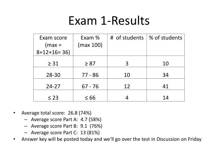
Exam 1-Results. Average total score: 26.8 (74%) Average score Part A: 4 .7 (58%) Average score Part B: 9.1 (76%) Average score Part C: 13 (81%) Answer key will be posted today and we’ll go over the test in Discussion on Friday. Lecture 11: Introduction to the Theory of the Firm.

E N D
Exam 1-Results • Average total score: 26.8 (74%) • Average score Part A: 4.7 (58%) • Average score Part B: 9.1 (76%) • Average score Part C: 13 (81%) • Answer key will be posted today and we’ll go over the test in Discussion on Friday
Lecture 11: Introduction to the Theory of the Firm Production in the short run
Theory of the firm (1) • Firm=producer=supplier=seller • How do firms decide how and how much to produce in order to maximize profit? • Firm’s decision has two components: • Production—how to combine inputs to produce outputs? • Cost – how do costs vary with output?
Theory of the firm (2) • The firm’s decision will depend on: • Time frame: short-run versus long-run • Market structure: • Perfect competition • Imperfect competition • Monopoly
Production Process or Function: The relationship that describes how inputs are combined to produce outputs Prices and money do not appear here. Production is a physical process
Categories of inputs or factors of production • Labor • Workers • Management/entreprenuership • Capital • Physical capital - machinery, equipment, buildings • Land is sometimes a separate input category, especially for agriculture • Materials - Inputs like energy, chemicals, plastic, and other materials
Categories of outputs or products • Goods • Pizzas, cars, buildings, clothes, computers, paintings • Services • Pizza delivery, medical exams, cleaning service, income tax preparation, rock concert • Both goods and services are outputs of production processes
In Class Assignment 1 • Name 3 inputs, at least 1 labor and 1 capital, required to produce a: • McDonald’s Happy Meal • Bicycle • Divorce decree • Vikings game • University of Minnesota graduate • BBQ in your back yard
In Class Assignment 1 – some examples of inputs • Name 3 inputs, at least 1 labor and at least 1 capital, required to produce a: • McDonalds Happy Meal (ingredients, equipment, workers, building) • Bicycle (parts, workers, equipment, building) • Divorce (lawyers, judge, office supplies, buildings) • Vikings game (players, stadium, referees) • University of Minnesota graduate (buildings, teachers, students) • BBQ in your back yard (backyard, food, grill)
In Class Assignment Follow Up • Which inputs would you need more of to go from producing 1 to producing 10 units?
Inputs that might change if production goes from 1 to 10 units • McDonalds Happy Meal -- ingredients, equipment, workers (per hour), building • bicycle -- parts, workers, equipment, building • Divorce (lawyers, judge, office supplies, buildings) • Vikings game –players, stadium, referees (if on different days) • University of Minnesota graduate (buildings, teachers, students) • BBQ in your back yard (backyard, food, grill)
Production function • Q = f (K, L) where Q is output; K is capital and L is labor Q Production surface = amount of Q produced with different combinations of K and L Q2 K Q1 L
Common functional forms for production functions • Cobb‐Douglas : Q = K0.7L0.5 • Quadratic : Q= 10L– L2+6K–0.3K2
Example: Cobb Douglas • Q = K0.7L0.5 • If K=10 and L=20, Q=10.7x 20.5= 22.4
Example: Cobb Douglas • Q = K0.7L0.5 • When both inputs increase…
Example: Cobb Douglas • Q = K0.7L0.5 • When only one input increases… 25.1-22.4 =2.7 15.8 -11.2 =4.6
Law of diminishing returns:if other inputs are fixed, the increase in output from an increase in the variable input must eventually decline.
Law of diminishing returns • Q = K0.7L0.5
Example: Quadratic • Q= 10L– L2+6K–0.3K2
Example: Quadratic • Q= 10L– L2+6K–0.3K2
Example: Quadratic • Q= 10L– L2+6K–0.3K2
Question: Why might total output decline when more inputs are added?
Production technology • “Production technology” describes the maximum quantity of output a firm can produce from a given quantities of inputs. Production function with 1 input
Production technology • Example: There are two restaurants selling identical sandwiches and pizzas. Firm 1 uses a conventional oven while firm 2 uses a “improved” oven. Their production functions are: • Firm 1: Q1 = 50K.5L.5 • Firm 2: Q2=100K.5L.5 • For the same K and L, Firm 2 will produce more Q
Technical change • Technical change: an advance in technology that allows more output to be produced with the same level of inputs. Examples: • Ovens that cook faster • Higher-yielding seed varieties • Faster, smaller computers
The Effect of Technological Progress in Food Production(Q= food production, L = labor)
Production in the short and long run • Refersto the time required to change inputs, holding technology constant • Not the same as technical change • Long run:the shortest period of time required to alter the amounts of all inputs used in a production process • Defined by the input that takes longest to change • Short run:the longest period of time during which at least one of the inputs used in a production process cannot be varied • If the long run is 5 years, the short run is less than 5 years
Fixed and variable inputs • Variable input:an input that can be varied in the short run • Fixed input:an input that cannot vary in the short run • Short and long run, and fixed and variable inputs vary for different products and producers
In Class assignment 2: Fill in the following table for: 1) McDonald’s Happy Meal and a University of Minnesota graduate
Fill in the following table for: University of Minnesota graduate
Short-run (SR) production • Production with at least one fixed input • Q= f(K , L) where Q is total output, K is the fixed input, and L is variable input • In SR, firm decides how much L to use given K. • Two key measures that firms can use to make decisions about how much L to use are: • Average product of labor: output per unit of labor • APL = Q/L • Marginal product of labor: the additional output produced from one addition unit of labor • MPL = ∂Q/∂L
Example-calculating AP and MP at a point • From previous example of Q = K0.7L0.5 • If K=10 and L=20, Q=10.7x 20.5= 22.4 • What are APL and MPL at that point? • APL = Q/L • Plug in values of K and L to get22.4/20 = 1.12 • MPL= ∂Q/∂L = .5K.7L -.5 • Plug in values for K and L: (.5)(10.7)(20-.5 )= (.5)(5)(.22) = .55
Q = K0.7L0.5 • If K=10 and L=20, Q=10.7x 20.5= 22.4 • What are APL and MPL at that point? • APL = Q/L= 22.4/20 = 1.12 • MPL= ∂Q/∂L = .5K.7L -.5 = (.5)(5)(.22) = .56 If L increases, will the APL go up or down? It will go down because if each additional unit is contributing less than the average (.56 < 1.12) , the average has to go down
Example- Calculating AP and MP in short run when K is fixed • Q = K0.7L0.5 • If Kis fixed at 10 and L is variable, what are APL and MPL? • APL = Q/L= (10.7L .5)/L = 5L.5/L • MPL= ∂Q/∂L = .5K.7L -.5 = (.5)(5) L -.5 = 2.5L -.5 If L increases, will the APL go up or down? It depends…
In class # 3 – Graph Q on one graph and MPL and APL on another, on the hand out
Relationship between MP and AP curves • When the marginal product curve lies above the average product curve, the average product curve must be rising • When the marginal product curve lies below the average product curve, the average product curve must be falling. • The two curves intersect at the maximum value of the average product curve.
Application of average v marginal: How should the police department allocate officers to maximize arrests per hour?
They should send 400 to West Philadelphia and 100 to City Center. Total arrests: 160+45+205