Download

1 / 8
80 likes | 182 Views
CS 290H Lecture 7 Symbolic factorization continued. No reading assignment for this Thursday We’ll talk about triangular solves, homework 2, and final projects Homework 2 due Thursday 28 Oct at 3 pm. 3. 7. 1. 6. 8. 10. 4. 10. 9. 5. 4. 8. 9. 2. 2. 5. 7. 3. 6. 1.

E N D
CS 290H Lecture 7Symbolic factorization continued • No reading assignment for this Thursday • We’ll talk about triangular solves, homework 2, and final projects • Homework 2 due Thursday 28 Oct at 3 pm
3 7 1 6 8 10 4 10 9 5 4 8 9 2 2 5 7 3 6 1 Elimination Tree G+(A) T(A) Cholesky factor • T(A) : parent(j) = min { i > j : (i, j) inG+(A) } • parent(col j) = first nonzero row below diagonal in L • T describes dependencies among columns of factor • Can compute G+(A) easily from T • Can compute T from G(A) in almost linear time
Describing the nonzero structure of L in terms of G(A) and T(A) • Let i > j. Then (i, j) is an edge of G+ iff j is an ancestor in T of some k such that (i, k) is an edge of G. [GLN 6.2.3]
Finding the elimination tree efficiently • Given the graph G = G(A) of n-by-n matrix A • start with an empty forest (no vertices) • for i = 1 : n add vertex i to the forest for each edge (i, j) of G with i > j make i the parent of the root of the tree containing j • Implementation uses a disjoint set union data structure for vertices of subtrees [GLN Algorithm 6.3 does this explicitly] • Running time is O(nnz(A) * inverse Ackermann function) • In practice, we use an O(nnz(A) * log n) implementation
Symbolic factorization: Computing G+(A) T and G give the nonzero structure of L either by rows or by columns. • Row subtrees[GLN Figure 6.2.5]: Tr[i] is the subtree of T formed by the union of the tree paths from j to i, for all edges (i, j) of G with j < i. • Tr[i] is rooted at vertex i. • The vertices of Tr[i] are the nonzeros of row i of L. • For j < i, (i, j) is an edge of G+ iff j is a vertex of Tr[i]. • Column unions[GLN Thm 6.1.5]: Column structures merge up the tree. • struct(L(:, j)) = struct(A(j:n, j)) + union( struct(L(:,k)) | j = parent(k) in T ) • For i > j, (i, j) is an edge of G+ iff either (i, j) is an edge of G or (i, k) is an edge of G+ for some child k of j in T. • Running time is O(nnz(L)), which is best possible . . . • . . . unless we just want the nonzero counts of the rows and columns of L
Finding row and column counts efficiently • First ingredient: number the elimination tree in postorder • Every subtree gets consecutive numbers • Renumbers vertices, but does not change fill or edges of G+ • Second ingredient: fast least-common-ancestor algorithm • lca (u, v) = root of smallest subtree containing both u and v • In a tree with n vertices, can do m arbitrary lca() computationsin time O(m * inverse Ackermann(m, n)) • The fast lca algorithm uses a disjoint-set-union data structure
Row counts [GLN Algorithm 6.12] • RowCnt(u) is # vertices in row subtree Tr[u]. • Third ingredient: path decomposition of row subtrees • Lemma: Let p1 < p2 < … < pk be some of the vertices of a postordered tree, including all the leaves and the root. Let qi = lca(pi , pi+1) for each i < k. Then each edge of the tree is on the tree path from pj to qj for exactly one j. • Lemma applies if the tree is Tr[u] and p1, p2, …, pk are the nonzero column numbers in row u of A. • RowCnt(u) = 1 + sumi ( level(pi) – level( lca(pi , pi+1) ) • Algorithm computes all lca’s and all levels, then evaluates the sum above for each u. • Total running time is O(nnz(A) * inverse Ackermann)
Column counts [GLN Algorithm 6.14] • ColCnt(v) is computed recursively from children of v. • Fourth ingredient: weights or “deltas” give difference between v’s ColCnt and sum of children’s ColCnts. • Can compute deltas from least common ancestors. • See GLN (or paper to be handed out) for details • Total running time is O(nnz(A) * inverse Ackermann)