Download
1 / 20
200 likes | 222 Views
Explore strategies to manage wireless media streaming for multiple users over time-varying channels while optimizing power consumption and playout quality. Utilize feedback mechanisms and power allocation techniques for efficient data transmission.

E N D
Inventory Control of Multiple Items Under Stochastic Prices and Budget Constraints David Shuman, Mingyan Liu, and Owen Wu University of Michigan INFORMS Annual Meeting October 14, 2009
Motivating Application: Wireless Media Streaming • Single source transmitting data streams to multiple users over a shared wireless channel • Available data rate of the channel varies with time and from user to user Key Features Two Control Objectives • Avoid underflow, so as to ensure playout quality • Minimize system-wide power consumption • Exploit temporal and spatial variation of the channel by transmitting more data when channel condition is “good,” and less data when the condition is “bad” • Challenge is to determine what is a “good” condition, and how much data to send accordingly Opportunistic Scheduling
Problem Description Timing in Each Slot • Transmitter learns each channel’s state through a feedback channel • Transmitter allocates some amount of power (possibly zero) for transmission to each user • Total power allocated in any slot cannot exceed a power constraint, P • Transmission and reception • Packets removed/purged from each receiver’s buffer for playing • Each user’s per slot consumption of packets is constant over time, dm • Transmitter knows each user’s packet requirements • Packets transmitted during a slot arrive in time to be played in the same slot • The available power P is always sufficient to transmit packets to cover one slot of playout for each user
Toy Example – Two Statistically Identical Receivers • Power constraint, P=12 • 3 possible channel conditions for each receiver: • Poor (60%) • Medium (20%) • Excellent (20%) Mobile Receivers User 1 Current Channel Condition: Medium Power Cost per Packet: 4 User 2 Base Station / Scheduler Current Channel Condition: Medium Power Cost per Packet: 4 0 5 8 5 Total Power Consumed: Time Remaining:
Toy Example – Two Statistically Identical Receivers • Power constraint, P=12 • 3 possible channel conditions for each receiver: • Poor (60%) • Medium (20%) • Excellent (20%) Mobile Receivers User 1 Current Channel Condition: Poor Power Cost per Packet: 6 User 2 Base Station / Scheduler • Current Channel Condition: Excellent • Power Cost per Packet: 3 8 4 20 4 Total Power Consumed: Time Remaining:
Toy Example – Two Statistically Identical Receivers • Power constraint, P=12 • 3 possible channel conditions for each receiver: • Poor (60%) • Medium (20%) • Excellent (20%) Mobile Receivers User 1 Current Channel Condition: Excellent Power Cost per Packet: 3 User 2 Base Station / Scheduler • Current Channel Condition: Poor • Power Cost per Packet: 6 20 3 29 3 Total Power Consumed: Time Remaining:
Toy Example – Two Statistically Identical Receivers • Power constraint, P=12 • 3 possible channel conditions for each receiver: • Poor (60%) • Medium (20%) • Excellent (20%) Mobile Receivers User 1 Current Channel Condition: Poor Power Cost per Packet: 6 User 2 Base Station / Scheduler • Current Channel Condition: Poor • Power Cost per Packet: 6 29 2 35 2 Total Power Consumed: Time Remaining:
Toy Example – Two Statistically Identical Receivers • Power constraint, P=12 • 3 possible channel conditions for each receiver: • Poor (60%) • Medium (20%) • Excellent (20%) Mobile Receivers User 1 Current Channel Condition: Poor Power Cost per Packet: 6 Reduced power cost per packet from 5.0 under naïve transmission policy to 4.1, by taking into account: (i) Current channel conditions (ii) Current queue lengths (iii) Statistics of future channel conditions User 2 Base Station / Scheduler • Current Channel Condition: Poor • Power Cost per Packet: 6 35 1 41 1 41 0 Total Power Consumed: Time Remaining:
Outline • Motivating Application: Wireless Media Streaming • Relation to Inventory Theory • Problem Formulation • Structure of Optimal Policy • Single Receiver • Two Receivers • Ongoing Work and Summary of Contributions
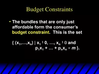
Relation to Inventory Theory • In inventory language, our problem is a multi-period, multi-item, discrete time inventory model with random ordering prices, deterministic demand, and a budget constraint • Items / goods → Data streams for each of the mobile receivers • Inventories → Receiver buffers • Random ordering prices → Random channel conditions • Deterministic demand → Users’ packet requirements for playout • Budget constraint → Transmitter’s power constraint
Related Work in Inventory Theory • Single item inventory models with random ordering prices (commodity purchasing) • B. G. Kingsman (1969); B. Kalymon (1971); V. Magirou (1982); K. Golabi (1982, 1985) • Kingsman is only one to consider a capacity constraint, and his constraint is on the number of items that can be ordered, regardless of the random realization of the ordering price • Capacitated single and multiple item inventory models with stochastic demands and deterministic ordering prices • Single: A. Federgruen and P. Zipkin (1986); S. Tayur (1992) • Multipe: R. Evans (1967); G. A. DeCroix and A. Arreola-Risa (1998); C. Shaoxiang (2004); • G. Janakiraman, M. Nagarajan, S. Veeraraghavan (working paper, 2009) • To our knowledge, no prior work on multiple items with stochastic pricing and budget constraints
Finite and Infinite Horizon Problem FormulationCost Structure, Information State, and Action Space • Linear ordering costs • is a random variable describing power consumption per unit of data transmitted to user m at time n • Linear holding costs • Per packet per slot holding cost hm assessed on all packets remaining in user m’s receiver buffer after playout consumption Cost Structure Information State • = vector of inventories (receiver queue lengths) at time n • = vector of prices (channel conditions) for slot n • Defined in terms of Yn, inventories (receiver queue lengths) afterordering • Must satisfy strict underflow constraints and budget (power) constraint Action Space
Finite and Infinite Horizon Problem FormulationSystem Dynamics, Optimization Criteria, and Optimization Problems • Stochastic prices independently and identically distributed across time, and independent across items System Dynamics • Finite horizon expected discounted cost criterion: Optimization Criteria • Infinite horizon expected discounted cost criterion: Optimization Problems
Single Item (User) CaseFinite Horizon Problem Dynamic Programming Equations • By induction, gn(•,c) convex for every n and c, with limy→∞ gn(y,c) = ∞ • If action space were independent of x, we would have a base-stock policy • Instead, we get a modified base-stock policy
Single Item (User) CaseStructure of Optimal Policy Theorem For every n {1,2,…,N} and c C, there exists a critical number,bn(c), such that the optimal control strategy is given by , where Furthermore, for a fixed n, bn(c) is nonincreasing in c, and for a fixed c: . Graphical representation of optimal ordering (transmission) policy Optimal Order Quantity Optimal Inventory Level After Ordering Inventory Level Before Ordering Inventory Level Before Ordering
Single Item (User) CaseOther Results • The basic modified base-stock structure is preserved if we: • Allow the holding cost function to be a general convex, nonnegative, nondecreasing function • Model the per item ordering cost (channel condition) as a homogeneous Markov process • Take the deterministic demand sequence to be nonstationary • Replace the strict underflow constraints with backorder costs • Complete characterization of the finite horizon optimal policy • If (i) the number of possible ordering costs (channel conditions) is finite, and • (ii) for every condition c, L(c):=P/(c•d) is an integer, • then we can recursively define a set of thresholds that determine the critical numbers • Process is far simpler computationally than solving the dynamic program • The infinite horizon optimal policy is the natural extension of the finite horizon optimal policy • Stationary modified base-stock policy characterized by critical numbers , where
Two Item (User) CaseStructure of Optimal Policy For a fixed vector of channel conditions, c, there exists an optimal policy with the structure below Inventory Level of Item 2 Before Ordering Inventory Level of Item 1 Before Ordering • Show by induction that at every time n, for every fixed vector of channel conditions c, gn(y,c) is convex and supermodular in y • bn(c1,c2) is a global minimum of gn(•,c)
Two Item (User) CaseComparison to Evans’ Problem Stochastic prices, fixed realization of c Deterministic prices (constant c), Evans, 1967 Inventory Level of Item 2 Before Ordering Inventory Level of Item 2 Before Ordering Inventory Level of Item 1 Before Ordering Inventory Level of Item 1 Before Ordering Two key differences: In addition to convexity and supermodularity, Evans showed the dominance of the second partials over the weighted mixed partials: - Without differentiability, strict convexity assumptions of Evans, can use submodularity of g in the direct value order (E. Antoniadou, 1996)
Two Item (User) CaseComparison to Evans’ Problem Stochastic prices, fixed realization of c Deterministic prices (constant c), Evans, 1967 Inventory Level of Item 2 Before Ordering Inventory Level of Item 2 Before Ordering Inventory Level of Item 1 Before Ordering Inventory Level of Item 1 Before Ordering Two key differences: In addition to convexity and supermodularity, Evans showed the dominance of the second partials over the weighted mixed partials: - Without differentiability, strict convexity assumptions of Evans, can use submodularity of g in the direct value order (E. Antoniadou, 1996) (ii) Different ordering costs lead to different target levels (global minimizers) Key takeaway: lower left region is not a “stability region,” making the problem harder
Ongoing Work and Summary Contribution to Wireless Communications • Analyze the specific streaming model • Introduce use of inventory models with stochastic ordering costs • Extend the literature on inventory models with stochastic ordering costs and budget constraints • No previous work with multiple items • Some results from models with stochastic demand, deterministic ordering costs “go through” in an adapted manner • e.g. single item modified base-stock policy, with one critical number for each price • However, some techniques and results do not go through • e.g., computation of critical numbers, direct value order submodularity of g in 2 item problem, “stability” region in 2 item problem Contribution to Inventory Theory • Numerical approximations and resulting intuition for general M-item problem • Piecewise linear convex ordering cost (finite generalized base-stock policy) • Average cost criterion Ongoing Work