Download
1 / 18
180 likes | 274 Views
Visual representations of networks. Judith Molka-Danielsen In765: Knowledge Networks Nov.08, 2005 Reference: Based on notes from “ Introduction to Social Network Methods ”, Robert A. Hanneman, UC,Riverside, 2001. Sampling Data on Relations.

E N D
Visual representations of networks Judith Molka-Danielsen In765: Knowledge Networks Nov.08, 2005 Reference: Based on notes from “Introduction to Social Network Methods”, Robert A. Hanneman, UC,Riverside, 2001.
Sampling Data on Relations • Full network methods – requires collecting info on each actor’s ties and with all actors. That is to take a census. Eg, count all shipments of X between all countries. Tells about the network structure (betweeness), but is expensive to collect data. Full network data allows for very powerful descriptions and analyses of social structures. Unfortunately, full network data can also be very expensive and difficult to collect. Obtaining data from every member of a population, and having every member rank or rate every other member can be very challenging tasks in any but the smallest groups.
Sampling Data on Relations • Snowball methods – used to track a special subset, Eg, business contacts, start with a group and ask them to name ties, it leaves out those not connected (isolates), can overstate connectedness, can miss connections (start snowball in wrong place), must start with chief.
Sampling Data on Relations • Ego-centric methods – start with several focal nodes, and ask who they are connected to, and see what of the focal nodes are connected to each other. Good for a large population, take a random sample, shows how individuals are embedded in neighborhoods, can determine how many connections, clustering. Cannot determine network distance, centrality. Can estimate network density, cliques, reciprocal ties.
Network characteristics • Size – number of nodes (k) • Number of relationships = k*k-1 (directed) and .5(k*k-1) for undirected. • Density – percentage of ties that could be present that actually are present. Highly dense networks have smaller distances. • Degree – sum of connections for a node • Reachability – there is a path to the node • Distance a-to-b – how many steps between two nodes. (walks, paths) • Geodesic distance – number of steps in the shortest path from one node to another node. • Diameter of a network – is the largest geodesic distance in the connected network. (longest-shortest path). • Eccentricity – is how far a node is from the furthest other node, or a nodes largest geodesic distance.
Connections between pairs of nodes Some applications (spreading rumors) do not just use the most efficient path (geodesic distance) but use all paths. • Maximum flow – how many nodes in a neighborhood of a source lead to pathways to a target. Strength of a tie to a node (target) is no stronger than the weakest link (no alternatives). (number of pathways, not just length is important) • Hubbell and Katz cohesion – count total connections between nodes, but weight according to length (longer is weaker). p.54 , or Taylor’s approach for a directed network and who usually sends or who receives.
Centrality and Power Power can be exerted in highly dense systems. It can be macro (system level, whole network) or micro (relational, between nodes). Systems as a whole can have power and power among actors may be unevenly distributed. • Degree • Closeness • Betweenness • Degree Centrality • Closeness Centrality • Betweenness Centrality • Flow Centrality
star, line and circle networks – degree, closeness, betweeness
Degree Centrality If an actor receives many ties, they are prominent, or to have high prestige. Actors who display high out-degree centrality are influential actors. What is the distribution of the actor's degree centrality scores? On the average, actors have a degree of 4.9, which is quite high, for 9 other actors.
Degree Centrality • Is the map homogeneous or hetrogeneous: calculating the coefficient of variation (standard deviation divided by mean, times 100) for in-degree and out-degree. By the rules of thumb used to evaluate coefficients of variation, the current values (35 for out-degree and 53 for in-degree) are moderate. Clearly, however, the population is more homogeneous with regard to out-degree (influence) than with regard to in-degree (prominence). • Freeman graph centralization measures: expresses the degree of inequality or variance in our network as a % of that of a perfect star network of the same size. In the current case, the out-degree graph centralization is 43% and the in-degree graph centralization 57% of these theoretical maximums. We would arrive at the conclusion that there is a substantial amount of concentration or centralization in this whole network. That is, the power of individual actors varies rather substantially, and this means that, overall, positional advantages are rather unequally distributed in this network
Closeness Centrality • Degree centrality only takes into account direct ties. • Closeness centrality approaches emphasize the distance of an actor to all others in the network by focusing on the geodesic distance from each actor to all others. • The sum of these geodesic distances for each actor is the "farness" of the actor from all others. • We can convert this into a measure of nearness or closeness centrality by taking the reciprocal (that is one divided by the farness) and normalizing it relative to the most central actor. • Actor 7 is most central (close), 2&5 next, 6 farthest. • In a small & high density net, centrality based on distance is very similar to centrality based on adjacency. • Again, can compare the variance in the actual data to the variance in a star network of the same size. This graph is very concentrated.
Betweeness Centrality • Betweenness centrality views an actor as being in a favored position to the extent that the actor falls on the geodesic paths between other pairs of actors in the network. If more people depend on me to make connections with other people, then I have more power. • Locate the geodesic paths between all pairs of actors, and to count up how frequently each actor falls in each of these pathways. If we add up, for each actor, the proportion of times that they are "between" other actors for the sending of information, we get the a measure of actor centrality. Normalized: this is % of the maximum possible betweenness that an actor could have. • Network centralization is relatively low. This makes sense, because one half of all connections can be made in this network without the aid of any intermediary -- hence there cannot be a lot of "between-ness." • In the sense of structural constraint, there is not a lot of "power" in this network. Actors #2, #3, and #5 appear to be relatively a good bit more powerful than others are by this measure.
*node data id gender role betweenness HOLLY female participant 78.33333588 BRAZEY female participant 0 CAROL female participant 1.333333373 PAM female participant 32.5 Jude female participant 39.5 JENNIE female participant 6.333333492 PAULINE female participant 12.mai ANN female participant 0.5 MICHAEL male participant 58.83333206 BILL male participant 0 LEE male participant 5 DON male participant 16.33333397 JOHN male participant 0 HARRY male participant 2.333333254 GERY male instructor 54.66666794 STEVE male instructor 16.83333397 BERT male instructor 13.66666698 RUSS male instructor 47.33333206 *Node properties ID x y color shape size shortlabel HOLLY 1160 271 255 1 10 HOLLY BRAZEY 1214 577 255 1 10 BRAZEY CAROL 671 612 255 1 10 CAROL PAM 985 127 255 1 10 PAM Jude 802 402 255 1 10 Jude JENNIE 729 187 255 1 10 JENNIE PAULINE 69 590 255 1 10 PAULINE ANN 877 818 255 1 10 ANN MICHAEL 182 224 255 1 10 MICHAEL BILL 380 137 255 1 10 BILL LEE 617 44 255 1 10 LEE DON 281 656 255 1 10 DON JOHN 617 839 255 1 10 JOHN HARRY 382 410 255 1 10 HARRY GERY 1051 706 255 1 10 GERY STEVE 64 394 255 1 10 STEVE BERT 348 812 255 1 10 BERT RUSS 1176 426 255 1 10 RUSS Node Data in Camptown.txt
Tie Data in Camptown.txt *Tie data from to friends strength HOLLY PAM 1 1 Jude HOLLY 1 2 PAULINE Jude 1 2 JOHN RUSS 1 3 HARRY HOLLY 1 2 HARRY MICHAEL 1 1 BERT RUSS 1 3 RUSS GERY 1 1 RUSS STEVE 1 3 RUSS BERT 1 2 HOLLY BRAZEY 0 7 HOLLY CAROL 0 17 BRAZEY PAULINE 0 7 BRAZEY ANN 0 6 BRAZEY MICHAEL 0 15 PAM MICHAEL 0 9 PAM BILL 0 16 PAM LEE 0 13 JENNIE BRAZEY 0 8 PAULINE JENNIE 0 5 PAULINE ANN 0 4 ANN Jude 0 7 ANN MICHAEL 0 9 BILL LEE 0 10 DON ANN 0 12