Download
1 / 27
270 likes | 336 Views
Learn how to use Hidden Markov Models (HMMs) to generate and evaluate sequences, compute probabilities, and implement algorithms like Forward, Backward, and Posterior Decoding. Explore topics like Viterbi algorithm, higher-order HMMs, and modeling state durations.

E N D
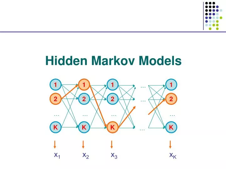
1 2 2 1 1 1 1 … 2 2 2 2 … K … … … … x1 K K K K x2 x3 xK … Hidden Markov Models
1 1 1 1 … 2 2 2 2 … … … … … K K K K … Generating a sequence by the model Given a HMM, we can generate a sequence of length n as follows: • Start at state 1 according to prob a01 • Emit letter x1 according to prob e1(x1) • Go to state 2 according to prob a12 • … until emitting xn 1 a02 2 2 0 K e2(x1) x1 x2 x3 xn
Evaluation We will develop algorithms that allow us to compute: P(x) Probability of x given the model P(xi…xj) Probability of a substring of x given the model P(i = k | x) “Posterior” probability that the ith state is k, given x A more refined measure of which states x may be in
The Forward Algorithm fk(i) = P(x1…xi, i = k) (the forward probability) Initialization: f0(0) = 1 fk(0) = 0, for all k > 0 Iteration: fk(i) = ek(xi) l fl(i – 1) alk Termination: P(x) = k fk(N)
Motivation for the Backward Algorithm We want to compute P(i = k | x), the probability distribution on the ith position, given x We start by computing P(i = k, x) = P(x1…xi, i = k, xi+1…xN) = P(x1…xi, i = k) P(xi+1…xN | x1…xi, i = k) = P(x1…xi, i = k) P(xi+1…xN | i = k) Then, P(i = k | x) = P(i = k, x) / P(x) Forward, fk(i) Backward, bk(i)
The Backward Algorithm – derivation Define the backward probability: bk(i) = P(xi+1…xN | i = k) “starting from ith state = k, generate rest of x” = i+1…N P(xi+1,xi+2, …, xN, i+1, …, N | i = k) = li+1…N P(xi+1,xi+2, …, xN, i+1 = l, i+2, …, N | i = k) = l el(xi+1) akli+1…N P(xi+2, …, xN, i+2, …, N | i+1 = l) = l el(xi+1) aklbl(i+1)
The Backward Algorithm We can compute bk(i) for all k, i, using dynamic programming Initialization: bk(N) = 1, for all k Iteration: bk(i) = l el(xi+1) akl bl(i+1) Termination: P(x) = l a0l el(x1) bl(1)
Computational Complexity What is the running time, and space required, for Forward, and Backward? Time: O(K2N) Space: O(KN) Useful implementation technique to avoid underflows Viterbi: sum of logs Forward/Backward: rescaling at each few positions by multiplying by a constant
Posterior Decoding P(i = k | x) = P(i = k , x)/P(x) = P(x1, …, xi, i = k, xi+1, … xn) / P(x) = P(x1, …, xi, i = k) P(xi+1, … xn | i = k) / P(x) = fk(i) bk(i) / P(x) We can now calculate fk(i) bk(i) P(i = k | x) = ––––––– P(x) Then, we can ask What is the most likely state at position i of sequence x: Define ^ by Posterior Decoding: ^i = argmaxkP(i = k | x)
Posterior Decoding • For each state, • Posterior Decoding gives us a curve of likelihood of state for each position • That is sometimes more informative than Viterbi path * • Posterior Decoding may give an invalid sequence of states (of prob 0) • Why?
Posterior Decoding x1 x2 x3 …………………………………………… xN • P(i = k | x) = P( | x) 1(i = k) = {:[i] = k}P( | x) State 1 P(i=l|x) l k 1() = 1, if is true 0, otherwise
Viterbi, Forward, Backward VITERBI Initialization: V0(0) = 1 Vk(0) = 0, for all k > 0 Iteration: Vl(i) = el(xi) maxkVk(i-1) akl Termination: P(x, *) = maxkVk(N) • FORWARD • Initialization: • f0(0) = 1 • fk(0) = 0, for all k > 0 • Iteration: • fl(i) = el(xi) k fk(i-1) akl • Termination: • P(x) = k fk(N) BACKWARD Initialization: bk(N) = 1, for all k Iteration: bl(i) = k el(xi+1) akl bk(i+1) Termination: P(x) = k a0k ek(x1) bk(1)
Higher-order HMMs • How do we model “memory” larger than one time point? • P(i+1 = l | i = k) akl • P(i+1 = l | i = k, i -1 = j) ajkl • … • A second order HMM with K states is equivalent to a first order HMM with K2 states aHHT state HH state HT aHT(prev = H) aHT(prev = T) aHTH state H state T aHTT aTHH aTHT state TH state TT aTH(prev = H) aTH(prev = T) aTTH
Similar Algorithms to 1st Order • P(i+1 = l | i = k, i -1 = j) • Vlk(i) = maxj{ Vkj(i – 1) + … } • Time? Space?
Modeling the Duration of States 1-p Length distribution of region X: E[lX] = 1/(1-p) • Geometric distribution, with mean 1/(1-p) This is a significant disadvantage of HMMs Several solutions exist for modeling different length distributions X Y p q 1-q
Solution 1: Chain several states p 1-p X Y X X q 1-q Disadvantage: Still very inflexible lX = C + geometric with mean 1/(1-p)
Solution 2: Negative binomial distribution Duration in X: m turns, where • During first m – 1 turns, exactly n – 1 arrows to next state are followed • During mth turn, an arrow to next state is followed m – 1 m – 1 P(lX = m) = n – 1 (1 – p)n-1+1p(m-1)-(n-1) = n – 1 (1 – p)npm-n p p p 1 – p 1 – p 1 – p Y X(n) X(1) X(2) ……
Example: genes in prokaryotes • EasyGene: Prokaryotic gene-finder Larsen TS, Krogh A • Negative binomial with n = 3
Solution 3: Duration modeling Upon entering a state: • Choose duration d, according to probability distribution • Generate d letters according to emission probs • Take a transition to next state according to transition probs Disadvantage: Increase in complexity of Viterbi: Time: O(D) Space: O(1) where D = maximum duration of state F d<Df xi…xi+d-1 Pf Warning, Rabiner’s tutorial claims O(D2) & O(D) increases
Viterbi with duration modeling emissions emissions Recall original iteration: Vl(i) = maxk Vk(i – 1) akl el(xi) New iteration: Vl(i) = maxk maxd=1…DlVk(i – d) Pl(d) akl j=i-d+1…iel(xj) F L d<Df d<Dl Pl Pf transitions xi…xi + d – 1 xj…xj + d – 1 Precompute cumulative values
A state model for alignment M (+1,+1) Alignments correspond 1-to-1 with sequences of states M, I, J I (+1, 0) J (0, +1) -AGGCTATCACCTGACCTCCAGGCCGA--TGCCC--- TAG-CTATCAC--GACCGC-GGTCGATTTGCCCGACC IMMJMMMMMMMJJMMMMMMJMMMMMMMIIMMMMMIII
Let’s score the transitions s(xi, yj) M (+1,+1) Alignments correspond 1-to-1 with sequences of states M, I, J s(xi, yj) s(xi, yj) -d -d I (+1, 0) J (0, +1) -e -e -AGGCTATCACCTGACCTCCAGGCCGA--TGCCC--- TAG-CTATCAC--GACCGC-GGTCGATTTGCCCGACC IMMJMMMMMMMJJMMMMMMJMMMMMMMIIMMMMMIII
Alignment with affine gaps – state version Dynamic Programming: M(i, j): Optimal alignment of x1…xi to y1…yjending in M I(i, j): Optimal alignment of x1…xi to y1…yj ending in I J(i, j): Optimal alignment of x1…xi to y1…yjending in J The score is additive, therefore we can apply DP recurrence formulas
Alignment with affine gaps – state version Initialization: M(0,0) = 0; M(i, 0) = M(0, j) = -, for i, j > 0 I(i,0) = d + ie; J(0, j) = d + je Iteration: M(i – 1, j – 1) M(i, j) = s(xi, yj) + max I(i – 1, j – 1) J(i – 1, j – 1) e + I(i – 1, j) I(i, j) = max d + M(i – 1, j) e + J(i, j – 1) J(i, j) = max d + M(i, j – 1) Termination: Optimal alignment given by max { M(m, n), I(m, n), J(m, n) }