Download
1 / 43

E N D
1. Image Enhancement � Frequency Domain Filter
School of Electronics & Information Engineering
Soochow University
2. 2 Image Enhancement - 3 Frequency vs. spatial domain
Different approaches
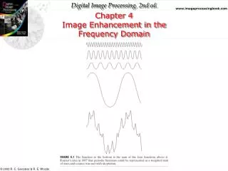
3. 3 1-D Discrete Fourier Transform f(x), x=0,1,�,M-1 . discrete function
F(u), u=0,1,�,M-1. DFT of f(x)
4. 4 2-D DFT 2-D: x-axis then y-axis
5. 5 Complex Quantities to Real Quantities Useful representation
6. 6 Some notes about 2-D Fourier transform Frequency axis
7. 7 DFT: example
8. 8 Fourier Transform FTTransform.mFTTransform.m
9. 9 Fourier Transform FTTransform.mFTTransform.m
10. 10 Fourier Transform FTTransform.mFTTransform.m
11. 11 Properties in the frequency domain Fourier transform works globally
No direct relationship between a specific components in an image and frequencies
Intuition about frequency
Frequency content
Rate of change of gray levels in an image
12. 12
13. 13 Image Enhancement - 3 Enhancement in frequency domain in principle is straightforward. However, it makes more sense to filter in the spatial domain using small filter masks.
The relationship between frequency and spatial domain is the convolution theorem
Select H(u,v) so that the desired image g(x,y) exhibits some highlighted features of f(x,y)
14. 14 Image Enhancement - 3
15. 15 Image Enhancement - 3
16. 16 Image Enhancement - 3 Lowpass filters
Ideal Lowpass filters
Butterworth Lowpass filters
Gaussian Lowpass filters
Highpass filters
Homomorphic filters
17. 17 Image Enhancement - 3 Ideal filters :
D(u,v) : distance from point (u,v) to the original
D0 : cutoff frequency
Ideal filter is nonphysical
Radially symmetric about the original
Special case : notch filter
Power ratio of enhanced and original image
If the image in question is of size MxN, its transform is of the same size. The center of the frequency rectangle is at (u,v) = (M/2, N/2) due to the fact that the transform has been centered. In this case, the distance from any point (u,v) to the center (original) of the Fourier transform is given by D(u,v) = [(u-M/2)2+(v-N/2)2]1/2. It is the Euclidean distance.If the image in question is of size MxN, its transform is of the same size. The center of the frequency rectangle is at (u,v) = (M/2, N/2) due to the fact that the transform has been centered. In this case, the distance from any point (u,v) to the center (original) of the Fourier transform is given by D(u,v) = [(u-M/2)2+(v-N/2)2]1/2. It is the Euclidean distance.
18. 18 Image Enhancement - 3
19. 19 Image Enhancement - 3
20. 20 Image Enhancement - 3
21. 21 Image Enhancement - 3
22. 22 Image Enhancement - 3
23. 23 Image Enhancement - 3 Butterworth lowpass filters A Butterworth filter of order 1 has no ringing. Ringing generally is imperceptible in filters of order 2, but can become a significant factor in filters of higher order.A Butterworth filter of order 1 has no ringing. Ringing generally is imperceptible in filters of order 2, but can become a significant factor in filters of higher order.
24. 24 Image Enhancement - 3 A Butterworth filter of order 2 with cutoff frequencies at radii of 5, 15, 30, 80, and 230.A Butterworth filter of order 2 with cutoff frequencies at radii of 5, 15, 30, 80, and 230.
25. 25 Image Enhancement - 3 A Butterworth filter of order 20 already exhibits the characteristics of the ILPF. A Butterworth filter of order 20 already exhibits the characteristics of the ILPF.
26. 26 Image Enhancement - 3 Guassian lowpass filters No ringing for all orders. Does not achieve as much smoothing as the Butterworth filter of order 2. This is an important characteristic in practice, especially in situations where any type of artifact is not acceptable.No ringing for all orders. Does not achieve as much smoothing as the Butterworth filter of order 2. This is an important characteristic in practice, especially in situations where any type of artifact is not acceptable.
27. 27 Image Enhancement - 3 No ringing for all orders. Does not achieve as much smoothing as the Butterworth filter of order 2. This is an important characteristic in practice, especially in situations where any type of artifact is not acceptable.No ringing for all orders. Does not achieve as much smoothing as the Butterworth filter of order 2. This is an important characteristic in practice, especially in situations where any type of artifact is not acceptable.
28. 28 Image Enhancement - 3
Ideal filters :
Butterworth highpass :
Gaussian lowpass :
29. 29 Image Enhancement - 3
30. 30 Spatial-domain HPF
31. 31 Ideal high-pass filters
32. 32 Butterworth high-pass filters
33. 33 Gaussian high-pass filters
34. 34 Laplacian frequency-domain filters Spatial-domain Laplacian (2nd derivative)
Fourier transform
35. 35 Laplacian frequency-domain filters
36. 36
37. 37
38. 38 Image Enhancement - 3 A simple image model: illumination�reflection model
f(x,y) : the intensity is called gray level for monochrome image
f(x,y)=i(x,y)*r(x,y)
0<i(x,y)<inf, the illumination
0<r(x,y)<1, the reflection
39. 39 Image Enhancement - 3 The illumination component
Slow spatial variations
Low frequency
The reflectance component
Vary abruptly, particularly at the junctions of dissimilar objects
High frequency
Homomorphic filters
Effect low and high frequency differently
Compress the low frequency dynamic range
Enhance the contrast in high frequency The illumination component of an image generally is characterized by slow spatial variations, while the reflectance component tends to vary abruptly, particularly at the junctions of dissimilar objects.
The net results of homomophic filtering is simultaneous dynamic range compression and contrast enhancement.The illumination component of an image generally is characterized by slow spatial variations, while the reflectance component tends to vary abruptly, particularly at the junctions of dissimilar objects.
The net results of homomophic filtering is simultaneous dynamic range compression and contrast enhancement.
40. 40 Image Enhancement - 3
41. 41 Image Enhancement - 3 f(x,y)=i(x,y)*r(x,y)
z(x,y)=ln f(x,y) = ln i(x,y) + ln r(x,y)
F{z(x,y)} = F{ln i(x,y)} + F{ln r(x,y)}
S(u,v) = H(u,v) I(u,v) + H(u,v) R(u,v)
s(x,y) = i�(x,y) + r�(x,y)
g(x,y) = exp[s(x,y)] = exp[i�(x,y)]exp[r�(x,y)]
42. 42 Image Enhancement - 3 The paramenters gamma_L and gamma_H are chosen so that gamma_L<1 and gamma_H>1. The curve shape can be approximated using the basic form of any of the ideal highpass filters. The paramenters gamma_L and gamma_H are chosen so that gamma_L<1 and gamma_H>1. The curve shape can be approximated using the basic form of any of the ideal highpass filters.
43. 43 Image Enhancement - 3 Gamma_L = 0.5, Gamma_H =2.0. A reduction of dynamic range in the brightness, together with an increase in contrast, brought out the details of objects inside the shelter and balanced the gray levels of the outside wall. The enhanced image is also sharper.Gamma_L = 0.5, Gamma_H =2.0. A reduction of dynamic range in the brightness, together with an increase in contrast, brought out the details of objects inside the shelter and balanced the gray levels of the outside wall. The enhanced image is also sharper.