Download

1 / 50
500 likes | 617 Views
Structure in the Experimental Treatments PGRM 11. Factors. Complex systems are affected by a wide range of factors : Ploughing system : soil type, ploughing depth, no of cultivations, type of plough, etc Animal production system : management regime, biological & environmental inputs

E N D
Factors Complex systems are affected by a wide range of factors: • Ploughing system: soil type, ploughing depth, no of cultivations, type of plough, etc • Animal production system: management regime, biological & environmental inputs • Ecological habitat: available food, cover light, temperature • Biochemical reaction: concentration of reagents, temperature, light
Factor Levels Enterprise type is a factor affecting farm outputs The different enterprise types considered are the levels of the factor:eg beef, beef suckler, dairy, mixed Levels may be categorical (as above), or quantitative as in the study of the effect of washing solution on retarding bacterial growth – these were 2%, 4% or 6%of an active ingredient. With quantitative levelsit makes sense to look for a trend (increasing or decreasing) in the response as the level increases.
Single factor experiments • Compare the mean response for the different levels of a single factor • Other factors affecting the response must be kept as constant as possible, and any affect of these will appear as random residual variation (due to the random allocation of units to the different levels of the factor) • The result will be: clear, valid but oflimited value Ex: comparing growth of lambs fed on 2 levels of protein supplement, we must use the same sources of protein for the two levels: we have no info what the response to protein level would be for other sources
(Multi)-factorial experiments Examine the effect of 2 (or more) factors at the same time Treatments:the various combinations of the levels of the different factors Ex:protein supplement: factor B (levels B1, B2, B3)protein source: factor A (levels A1, A2) 6 treatments A1B1, A1B2, A1B3 A2B1, A2B2, A2B3
Simple and Main effects • Simple effects of source: Difference (in mean growth) between source A1 & A2 can be considered at each of the 3 levels of protein. • Simple effects of protein: Differences between B1 & B2, B2 & B3 and between B3 & B1 can be measured for each source. • Main effects are averages of simple effects, and are not always meaningful
Example Note:the main effect of A, (1 + 1 + 7)/3, is also the difference between the MARGINAL means Here the effect of A depends on the level of B This is an INTERACTION between the factors A and B
Important Rule With an AB interaction:the effect of Achanges as the level of B changes Hence:averaging the effects of A over the levels of B makes no sense • The main effect of a factor can not be uncritically interpreted as the effect of the factor if there is an interaction • In this case report the ab treatment means and some meaningful comparisons, and not the separate means for levels of A and B
Why do factorial? • Factorial experiments compare a set of treatments which have a certain structure:the treatments simply consist of combinations of levels of 2 (or more) factors • so we already know how to do the analysis! • the factorial treatment structure will dictate sensible comparisons to make • The gain: • knowing whether the effect of one factor varies with the level of another • saving resources when there is no interaction,since a simple effect can be estimated at each level of the other factor and the results combined
Why the gain (in absence of interaction) A effect: since this is the same for all levels of B it is measured by the difference in the marginal means, each based on 18 observations. B effects: each B effect (B1vB2, B2vB3, B3vB1) is measured using means of 12 observations
Separate experiments (same resources) A effect: now measured by the difference between meansof 9 observations (was 18). B effects: now measured by the difference between means of 6 observations (was 12). Also: we don’t know if the A effects depend on the level of B – MORE LOSS OF INFORMATION!
PGRM pg 11-6 The enormous benefits (of factorial designs) arise through no extra cost but merely by reorganising the work programme. You can choose to get much more information for the same money or reduce the cost of achieving a given level of information.
SAS OUTPUT • ANOVA table • Table of MEANS with SED • Writing a summary
ANOVA ab factorial, replication r • Treat this as a 1-way structure, with ab treatments • Now partition the treatment SS, TSS
Example: time to development of Fasciola hepatica eggs under 2 combinations of temperature and relative humidity p<0.001 ***p<0.01 **p<0.05 *
Tables of Means Humidity effect:sig. when temp = 16 (7.4)non-sig. when temp = 22 (1.4) Temp. effect:sig. (12.0 & 18.0) at both levels of humidity SED = 1.49 Temperature Humidity Interpretation Overall treatments differ: F = 75.83 Interaction is significant: F = 8.1, so we really should examine the 4 means as above, and ignore the tests for main effects which eg compare levels of HUMIDITY averaged over levels of TEMP However, in this case, the TEMP effect is much larger than the interaction, its averaged effect broadly reflects its effect at each level of HUMIDITY
proc glm data = fasciola; class temp humidity; model time = temp humidity temp*humidity; lsmeans temp; lsmeans humidity; lsmeans temp*humidity; estimate ‘SED for temp’ temp 1 -1; estimate ‘SED for humidity’ humidity 1 -1;quit;proc glm data = fasciola; class temp humidity; model time = temp*humidity; estimate ‘SED tment means’ temp*humidity 1 -1;quit; One-way analysis Main effects & interaction SAS/GLM for 2-way analysis
Data must contain response values (time) in a single column identified by factor levels in 2 other columns This gives 3 variables (columns) for SAS program SAS demo! faciola.sas
What to present (again!) • Since the interaction is significant don’t report the main effects. • Present: • the 2-way table: (with SED) • a summary:the temp/humidity interaction was significant (p = 0.02)humidity effects were significant at temp = 16 (p = 0.0012)but not at temp = 22 (p = 0.40)temp effects were significant at both humidities (p < 0.0001), and greater when humidity = 1 SED = 1.49
Factorial experiment laid out in blocks • Above has laid out the ab treatments as a completely randomised design using rab experimental units (r for each treatment)Think: how would this be done in practice? • If we block the experimental units into blocks of size ab and randomly allocate the ab treatments to the units in the block we can then remove BSS from RSS, hopefully reducing it sufficiently to compensate for the reduction in DF • See example over …
2-way experiment laid out in blocks • Factor A: 2 levels Factor B: 3 levels • 60 experimental units available (10 per treatment) • Completely randomised design (CR): randomly allocate treatments of unitsRandomised blocks (RB): Group units into blocks of size 6 (so 10 blocks) & randomise the 6 treatments in each block, which may be much easier to do ANOVA
Practical: 4.2 Two-Factor Factorial Example 2 Bacterial count in sausages stored at 4 temperatures using 3 type of preservative methods
More than 2 factors! 3×4×5 experiment:ie Factors A, B, C with 3, 4,and 5 levels respectivelygiving 60 treatment combinations! The 3-factor ABC interaction measures how the 2-factor AB interaction changes over the levels of C(see over) Can get away with replication r = 1 provided the 3-factor interaction can be assumed negligible– not usually liked by journal editors! With r > 1 we include:main effects: A, B, C2-factor interactions: BC, CA, AB3-factor interaction: ABC
3-factor interaction for a 2×2×2 expt With C1: A effect is least at B2 With C2: A effect is largest at B2 Direction of A effect is different for C1, C2 AB interaction different a two C levels
3-factor interaction arising naturally See PGRM Fig 11.2.2 (b)
Examples – measuring the benefit • 2222: artificial insemination involving 256 heifers(r = 16 per treatment) • 345: imaginary example to practice calculating sample sizes! 120 units(r = 2) • 222: machine tool lifetime 24 units(r = 3)
Example 2x2x2x2 factorial Artificial insemination 256 heifers (64 each week) 4 factors at 2 levels. Compare precision A) 32 animals per treatment. SED = (2 s2/32) = s/4 where s2 = MSE. B) 128 animals for each level of a factor SED = (2 s2/128) = s/8. choices A) 4 experiments (r=32) B) 2 x 2 x 2 x 2 factorial (r=16 per combination) Plus With B all interactions can be estimated
Conclusion • Summary - The factorial design • - Halves the SED and quarters the number of animals required for a given level of precision • - Allows more general interpretation of the factor effects since they are tested over a wide range of levels of the other factors • - Allows a test of whether the factors interact. Compare precision A) 32 animals per treatment. SED = (2 s2/32) = s/4 where S2 = MSE. B) 128 animals for each level of a factor SED = (2 s2/128) = s/8.
3×4×5 expt with factors A, B, C & replication 2(120 units) For any factor not involved in a significant interaction Replication of Main effect means A B C 40 30 24 Replication of means in Interaction table, eg BC B C 1 2 3 4 5 Total 1 6 6 6 6 6 30 2 6 6 6 6 6 30 3 6 6 6 6 6 30 4 6 6 6 6 6 30Total 24 24 24 24 24 120 All interactions AB AC BC Treat Comb. 10 8 6 2 For comparing BC effects if only significant interaction is BC All 2-factor interactions significant, 3-factor not
Example An engineer is interested in the effects of cutting speed (A), tool geometry (B) and cutting angle (C)on the life (in hours) of a machine tool. Two levels of each factor are chosen,and three replicates of a 23 factorial design are run. Design: 2×2×2 No. treatments: 8 No. units: 24
Example: Data A B C LIFE(hr) Replicate 1 2 3 1 1 1 22 31 25 2 1 1 32 43 29 1 2 1 35 34 50 2 2 1 55 47 46 1 1 2 44 45 38 2 1 2 40 37 36 1 2 2 60 50 54 2 2 2 39 41 47
Example: ANOVA • Note: • ABC interaction non-significant • AC is only significant 2-factor interaction
Tables of MEANS SED = 4.48 Help!
Making sense of tables • From this analysis, the only terms that are significant are the B and C main effects and the AC interaction. • Thus, the only tables that need to be presented are the B main effect table and the AC tables of means. • Geometry (B) has a large effect, increasing the life by over 10 hours. • Cutting angle (C) increases the life considerably at low but not at high speed (A). • Another way of looking at the AC interaction is that increased speed increase tool life for the first cutting angle but reduces it for the second cutting angle.
SAS/GLM code proc glm data = mydataset; model response = a b c b*c c*a a*b a*b*c; lsmeans a b c b*c c*a a*b a*b*c; quit; Is this the best we can suggest? With one (AC) significant interaction lsmeans b a*c / stderr; estimate ‘b SED’ b 1 -1; /* ac SED = sqrt(2) x stderr */
Calculating SEDs Recall (with equal replication): SED = √2 × SEM SED: standard error of a difference SEM: standard error of a mean SAS: lsmeans B / stderr; lsmeans A*C / stderr; lsmeans A*B*C / stderr; will give SEM, & a usually useless p-value testing whether the mean is 0! f3_toolLife.sas
Calculating SED: For the AC interaction: SEM = 2.2422707NB: usual SAS unhelpful precision! so SED = 1.414 × 2.2422707 = 3.17 (3 sig. figs.)
Transformations of data Analysing log(response)
Interpreting the log scale Linear relationshiplog(y) = a + bx (here: log = log2)y = 2a+ bx = 2a 2bx Compare y-values for a unit increase in x,ie y1 at x and y2 at x + 1 y2 / y1 = [2a 2(bx + b)]/ [2a 2bx] = 2b Increasing x by 1, multiplies y by 2b eg if b = -1 this is a 50% decrease in y
Understanding the LOG scale • where effects of a variate are proportional Example: • uses log2 (logs to base 2) • slope b = -1 • giving a 50% decrease per unit increase in x
Dilution of drug in milk Excretion of sodium penicillin for five milkings for a cow. Relationship is not linear.
LOG-scale Slope b= -2.14 exp(-2.14) = 0.12 Conclusion: Each milking reduces the# units to 12% of previous milking
Revision: t-test, p-value, significance level, hypothesis testing, and much more ALL IN ONE OVERHEAD!
H0: = 0 t = ESTIMATE/SE t-test eg =3 - 1 1 - 22 +3 regression slope When H0 is true: 5% of t-values fall on axis below blue shading – for 11 df: beyond ±2.2 For given t, V, p is proportion of more extreme values