Download
1 / 28
280 likes | 387 Views
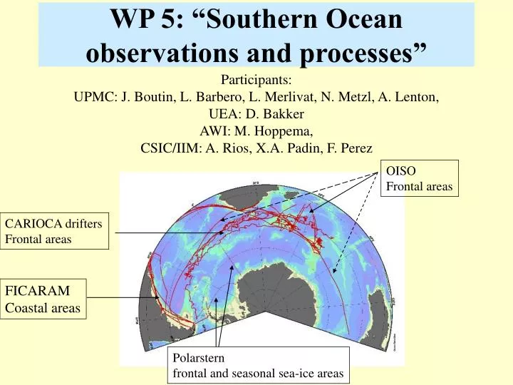
WP 5: “Southern Ocean observations and processes”. Participants: UPMC: J. Boutin, L. Barbero, L. Merlivat, N. Metzl, A. Lenton, UEA: D. Bakker AWI: M. Hoppema, CSIC/IIM: A. Rios, X.A. Padin, F. Perez. OISO Frontal areas. CARIOCA drifters Frontal areas. FICARAM Coastal areas.

E N D
WP 5: “Southern Ocean observations and processes” Participants: UPMC: J. Boutin, L. Barbero, L. Merlivat, N. Metzl, A. Lenton, UEA: D. Bakker AWI: M. Hoppema, CSIC/IIM: A. Rios, X.A. Padin, F. Perez OISO Frontal areas CARIOCA drifters Frontal areas FICARAM Coastal areas Polarstern frontal and seasonal sea-ice areas
WP5 Objectives • To assess the air-sea CO2 flux and its space and time variability in specific sink regions of the Atlantic and Indian sectors of the Southern Ocean. • Coastal regions: seasonal variability • Frontal regions: seasonal to decadal variability • To understand processes responsible for the observed variability of the air-sea CO2 flux • Seasonal sea-ice regions • Enhanced CO2 uptake close to islands • Net community production in frontal regions • Influence of stratospheric ozone on the observed decadal variability • To provide inputs for estimating air-sea CO2 fluxes at regional and monthly time scales to constrain atmospheric inverse modelling. • New set of measurements incorporated in the Takahashi et al. (2009) climatology • Revised estimates of air-sea CO2 flux integrated in the SAZ
WP5 Objectives • To assess the air-sea CO2 flux and its space and time variability in specific sink regions of the Atlantic and Indian sectors of the Southern Ocean. • Coastal regions: seasonal variability • Frontal regions: seasonal to decadal variability • To understand processes responsible for the observed variability of the air-sea CO2 flux • Seasonal sea-ice regions • Enhanced CO2 uptake close to islands • Net community production in frontal regions • Influence of stratospheric ozone on the observed decadal variability • To provide inputs for estimating air-sea CO2 fluxes at regional and monthly time scales to constrain atmospheric inverse modelling. • New set of measurements incorporated in the Takahashi et al. (2009) climatology • Revised estimates of air-sea CO2 flux integrated in the SAZ
FICARAM cruises: coastal region A. Rios, X.A. Padin See poster 7
South American Shelf South Atlantic Convergence Falkland Current Strongest sink! 2001 2008 2001 2008 2001 2008 =>The majority of provinces in the Patagonian Sea behaved as an intense sink of CO2 during autumn and spring, in particular the oceanic waters of the SAC province (South Atlantic Convergence zone 40 ºS–51 ºS) :-5.4±3.6 mol m-2 yr-1 =>The Antarctic waters in the Drake Passage were found to be CO2 undersaturated during the boreal autumn (Padin et al. 2009)
J. Boutin, L. Merlivat, L. Barbero (UPMC) CARIOCA drifters in the frontal regions STF 83 months of hourly measurements (CO2 fugacity and auxiliary parameters) acquired by 7 CARIOCA drifters in the Southern Atlantic and Indian Ocean during 4 seasons. SAF Combining part of this data set with older Carioca data in other sectors of the Southern Ocean, SAZ sink estimated to be 0.8PgC yr-1 (Boutin et al., 2008) but large unknowns in the Pacific SAZ (the largest estimated sink: 0.5PgC yr-1)
CARIOCA + Ship data in Pacific SAZ => air-sea CO2 source in regions of deep water formations 0 -100 -200 -300 -400 -500 Fit for SST=6°C Fit for MLD=50m MLD (m) Fit for SST=10°C 2020 2060 2100 2140 DIC (µmol/kg) DIC vs. Climatological MLD (Dong et al. 2008) Deep MLD – Rich DIC DIC = a + b*MLD – c*SST σ = 9.7 µmol/kg For |MLD| > 100m: DIC σ = 5.8 µmol/kg DIC = f(SST,MLD) AT = f(SST,SSS) (SST and SSS from WOA) pCO2
ΔpCO2 in July Our study (1x1° grid): Takahashi, 2009 (4x5° grid): McNeil, 2007 (June, July, August) (1x1° grid):
Annual flux 2005, SAZ Pac., same k, quickscat wind speed Barbero et al. 2009 -0.04 Pg C y-1 Takahashi et al. 2009 -0.16 Pg C y-1 McNeil et al. 2007 -0.5 Pg C y-1 Barbero Takahashi Mc Neil Boutin Boutin et al. 2008 -0.5 Pg C y-1 Barbero et al. 2009, in prep.
Decadal variations of fCO2 in the Southern Ocean (OISO Cruises) Nicolas Metzl and Andrew Lenton (UPMC) Trend atmosphere: + 1.7 µatm/yr Trend ocean: + 2.1 µatm/yr Ocean sink decreases ? : -0.4 µatm/yr Observations suggest a recent stabilization of the CO2 uptake in the Southern Ocean All data 1991-2008 in SOCAT and CDIAC Metzl, DSR, 2009
Exploring fCO2 trends in four selected regions and for summer and winter Cruises: 1991-1995 (MINERVE) and 1998-2007 (OISO)
Summer and winter ocean fCO2 trends (µatm/yr) in four regions in the Southern Indian Ocean (1991-2007) Average: 2.1 (+0.3) µatm/yr (same as moon view) Summer Winter Atm. Metzl, DSR 2009 Almost always above the atmospheric CO2 rate Mainly explained by import of DIC from subsurface linked to positive phase of the SAM.
O3 clim: ocean CO2 sink increases, Ocean pCO2: +1.1 uatm/yr O3 hole: ocean CO2 sink stabilized Ocean pCO2: +2.0 µatm/yr Air-sea CO2 fluxes in the Southern Ocean Results from a coupled climate/carbon model (IPSL/LOOP with and without O3 hole) (Lenton et al, GRL, 2009)
WP5 Objectives • To assess the air-sea CO2 flux and its space and time variability in specific sink regions of the Atlantic and Indian sectors of the Southern Ocean. • Coastal regions: seasonal variability • Frontal regions: seasonal to decadal variability • To understand processes responsible for the observed variability of the air-sea CO2 flux • Seasonal sea-ice regions • Enhanced CO2 uptake close to islands • Net community production in frontal regions • Influence of stratospheric ozone on the observed decadal variability • To provide inputs for estimating air-sea CO2 fluxes at regional and monthly time scales to constrain atmospheric inverse modelling. • New set of measurements incorporated in the Takahashi et al. (2009) climatology • Revised estimates of air-sea CO2 flux integrated in the SAZ
Seasonal sea-ice region:High fCO2 and DIC below sea ice, low values upon ice melt. fCO2(w-a) (µatm) Ice concentration (fraction) fCO2(w-a) (µatm) 14/01 03/12 Oceanic CO2 source potential Oceanic CO2 sink potential Why? 21/12 07/12 FS Polarstern, ANT 20-2, 03/12/2002-14/01/2003 07/01 15/12 30/12 Below ice: fCO2(w-a) 0 to 40 µatm Upon melt: fCO2(w-a) -50 to 0 µatm Bakker et al., Biogeosciences, 2008
High fCO2 and DIC below sea ice by entrainment of ‘old’ CO2-rich Warm Deep Water Below sea ice: fCO2(w-a) of 0 - 40 µatm. The ice mostly (?) stops outgassing of CO2 (Bakker et al., 2008). N.B. Air-sea ice CO2 fluxes are important (Delille et al., Nomura et al. @ ICDC8). Dissolved inorganic carbon (µmol/kg) High DIC at 50 m depth
Rapid reduction of surface fCO2 during and upon ice melt 0°W Surface fCO2 decrease during ice melt 08-10/12/2004 20/12/2004 Sea ice cover Brown ice, 17-20/12/02 (%) Below ice: fCO2(w-a) 0 to 40 µatm Upon melt: fCO2(w-a) -50 to 0 µatm Biological carbon uptake rapidly creates a CO2 sink during and upon ice melt. 17/12/2004 The Weddell Gyre may well be an annual CO2 sink (Bakker et al., 2008). This supports the role of Antarctic sea ice on glacial-interglacial CO2 variations (Stephens and Keeling, 2000).
The island mass effect and biological carbon uptake for the Crozet Plateau DIC deficit in the upper 100 m (Bakker et al., 2007, DSR II) SOUTH: HNLC, upstream of the plateau Little air-sea CO2 transfer; DIC deficit 1 mol/m2 Are HNLC waters more productive than we think? NORTH: Crozet bloom, downstream of the plateau Sink for atmospheric CO2; DIC deficit 2-3 mol/m2; How important are such blooms for Southern Ocean carbon export?
During some periods (with no salinity or temperature variations (except diurnal variation)), diurnal variation of DIC (max. at sunrise, min. at sunset) and high fluorescence indicate large biological activity. The day-to-day decrease of the DIC maximum at the end of the night provides an estimate of the net community production in the mixed layer Net community production derived from CARIOCA hourly measurements ~Net community production in the mixed layer – air-sea flux DIC Sunrise Sunset See poster 5 (Boutin & Merlivat, GRL, 2009)
SAF PF Estimating biological carbon production rates by an in situ non-intrusive method using CARIOCA measurements (Boutin & Merlivat, GRL, 2009). November-December March April In nov-dec., in SAZ of eastern Atlantic, 0.3<NCP<0.6 mmol kg-1 d-1 In march-april, close to polar front in western Atlantic: 1.4< NCP < 2.9 mmol kg-1 d-1 Main avantages of the method: - non-intrusive method, - compared to in situ O2/Argon method, the contribution of air-sea flux is small with respect to biological contribution - provides an estimate of NCP averaged over a few days in the mixed layer
Main results • Increased number of surface CO2 measurements in the Southern Atlantic and Indian Oceans (open and coastal regions) from ships and CARIOCA drifters. • With respect to Takahashi et al. (2009) climatology, SAZ sink in the Southern Ocean could be reduced by 0,1 Pg C yr-1 when taking into account outgassing in regions of deep water formation. • On a decadal scale, surface ocean CO2 fugacity increases at a rate almost always above the atmospheric rate in the Southern Indian Ocean (1991-2007). In agreement with simulations of a coupled model including stratospheric ozone depletion. • Large phytoplankton blooms downstream of the Crozet and Kerguelen islands and in coastal areas create a strong sink for atmospheric CO2. • Large variability of air-sea CO2 flux close to sea ice • New methodology developped to estimate in situ carbon biological production from CARIOCA drifters
Future needs/ Remaining questions • Maintain repetitive tracks to monitor long term trends: is the southern ocean sink decreasing or not? • Deepen process studies based on Carboocean acquired measurements: among others: • New in situ estimates of carbon biological production from all CARIOCA drifters: • Impact of mesoscale variability on fCO2 measurements • CO2 variability in seasonal sea ice regions • .....
Thanks to :-WP5 participants for fruitful and constructive work-Benjamin for helping in data synthesis-Andrea for helping in the workshops organisation-Andy and Christoph for coordination
South American Shelf South Atlantic Convergence Falkland Current Strongest sink! 2001 2008 2001 2008 2001 2008 Figure 5: Temporal variation of the averaged SST, SSS, chl-a, WS, fCO2 and FCO2 cruise (error bars stand for the respective standard deviation) in SAS (South American Shelf 31ºS S–40ºS), SAC (South Atlantic Convergence zone 40 ºS–51 ºS), and FC (Falkland Current 51 ºS–56 ºS). Spring and autumn values are shown as squares and circles, respectively. Significant regression lines (p<0.05) and regression slopes including the standard error are also given. Solid lines stand for spring results and dashed lines for autumn. =>The majority of provinces in the Patagonian Sea behaved as an intense sink of CO2 during autumn and spring, in particular the oceanic waters of the SAC province (South Atlantic Convergence zone 40 ºS–51 ºS) :-5.4±3.6 mol m-2 yr-1 =>The Antarctic waters in the Drake Passage were found to be CO2 undersaturated during the boreal autumn (Padin et al. 2009)
Buoy and ship trajectories in the South Pacific SAZ STF SAF CARIOCA 01110 April/2004-April/2005 CARIOCA 03740 April/2004-June/2005 Palmer cruises April-May/2004 March/2005 September/2005 September/2006 • Subtropical Front (STF): Climatological (Orsi et al.,1995, Deep Sea Res.) • Subantarctic Front (SAF): Altimetry data (Sallée et al., 2008, J. Climate)
Conclusions: • Method for the estimation of air-sea CO2 fluxes from MLD, SST and SSS in the SAZ of the Southern Pacific Ocean. • Large variability in DIC during the summer months due to biological production. • No direct correlation between NCP and SEAWIFS-MODIS colour images for weak Chl concentrations. • Method validated against independent measurements (1979-2008) • The Pacific SAZ is a weaker sink than estimated by other methods. For more info: Leticia.Barbero@locean-ipsl.upmc.fr
Schematic principle of NCP estimation from observed diurnal variation of DIC: a DIC minimum at sunset and a DIC maximum at sunrise together with significant fluorescence and no change in salinity (also alkalinity). a warm diurnal layer is formed during the daylight period during the second part of the day, nocturnal convection mixes the warm layer within the mixed layer (surface buoyancy flux) Diagram showing depth zones in a typical mixed layer cycle (Brainerd and Gregg, DSR 1,1995)
From ice covered CO2–rich waters to a biologically mediated CO2 sink upon ice melt in the eastern Weddell Gyre Dorothee Bakker, Mario Hoppema, Mike Schröder, Walter Geibert, Hein de Baar School of Environmental Sciences, University of East Anglia, Norwich, U.K. Alfred Wegener Institute for Polar and Marine Research, Bremerhaven, Germany Earth Science, School of Geosciences, University of Edinburgh, U.K. Royal Netherlands Institute for Sea Research, Texel, The Netherlands Funding from EU CarboOcean, the Royal Society and NERC CASIX