Download

1 / 32
320 likes | 609 Views
Additive Models, Trees, etc. Based in part on Chapter 9 of Hastie, Tibshirani, and Friedman David Madigan. Predictive Modeling. Goal: learn a mapping: y = f ( x ; ) Need: 1. A model structure 2. A score function 3. An optimization strategy

E N D
Additive Models, Trees, etc. Based in part on Chapter 9 of Hastie, Tibshirani, and Friedman David Madigan
Predictive Modeling Goal: learn a mapping: y = f(x;) Need: 1. A model structure 2. A score function 3. An optimization strategy Categorical y {c1,…,cm}: classification Real-valued y: regression Note: usually assume {c1,…,cm} are mutually exclusive and exhaustive
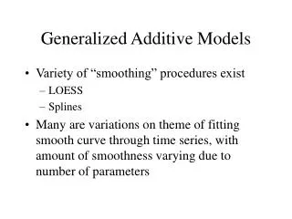
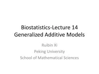
Generalized Additive Models • Highly flexible form of predictive modeling for regression and classification: • g (“link function”) could be the identity or logit or log or whatever • The f s are smooth functions often fit using natural cubic splines
Basic Backfitting Algorithm arbitrary smoother - could be natural cubic splines
Example using R’s gam function library(mgcv) set.seed(0) n<-400 x0 <- runif(n, 0, 1) x1 <- runif(n, 0, 1) x2 <- runif(n, 0, 1) x3 <- runif(n, 0, 1) pi <- asin(1) * 2 f <- 2 * sin(pi * x0) f <- f + exp(2 * x1) - 3.75887 f <- f + 0.2 * x2^11 * (10 * (1 - x2))^6 +10 * (10 * x2)^3 * (1 - x2)^10 - 1.396 e <- rnorm(n, 0, 2) y <- f + e b<-gam(y~s(x0)+s(x1)+s(x2)+s(x3)) summary(b) plot(b,pages=1) http://www.math.mcgill.ca/sysdocs/R/library/mgcv/html/gam.html
Tree Models • Easy to understand: recursively divide predictor space into regions where response variable has small variance • Predicted value is majority class (classification) or average value (regression) • Can handle mixed data, missing values, etc. • Usually grow a large tree and prune it back rather than attempt to optimally stop the growing process
Training Dataset This follows an example from Quinlan’s ID3
Output: A Decision Tree for “buys_computer” age? <=30 overcast >40 30..40 student? credit rating? yes no yes fair excellent no yes no yes
Algorithms for Decision Tree Induction • Basic algorithm (a greedy algorithm) • Tree is constructed in a top-down recursive divide-and-conquer manner • At start, all the training examples are at the root • Attributes are categorical (if continuous-valued, they are discretized in advance) • Examples are partitioned recursively based on selected attributes • Test attributes are selected on the basis of a heuristic or statistical measure (e.g., information gain) • Conditions for stopping partitioning • All samples for a given node belong to the same class • There are no remaining attributes for further partitioning – majority voting is employed for classifying the leaf • There are no samples left
Information Gain (ID3/C4.5) • Select the attribute with the highest information gain • Assume there are two classes, P and N • Let the set of examples S contain p elements of class P and n elements of class N • The amount of information, needed to decide if an arbitrary example in S belongs to P or N is defined as e.g. I(0.5,0.5)=1; I(0.9,0.1)=0.47; I(0.99,0.01)=0.08;
Information Gain in Decision Tree Induction • Assume that using attribute A a set S will be partitioned into sets {S1, S2 , …, Sv} • If Si contains piexamples of P and ni examples of N, the entropy, or the expected information needed to classify objects in all subtrees Si is • The encoding information that would be gained by branching on A
Class P: buys_computer = “yes” Class N: buys_computer = “no” I(p, n) = I(9, 5) =0.940 Compute the entropy for age: Hence Similarly Attribute Selection by Information Gain Computation
Gini Index (IBM IntelligentMiner) • If a data set T contains examples from n classes, gini index, gini(T) is defined as where pj is the relative frequency of class j in T. • If a data set T is split into two subsets T1 and T2 with sizes N1 and N2 respectively, the gini index of the split data contains examples from n classes, the gini index gini(T) is defined as • The attribute provides the smallest ginisplit(T) is chosen to split the node
Avoid Overfitting in Classification • The generated tree may overfit the training data • Too many branches, some may reflect anomalies due to noise or outliers • Result is in poor accuracy for unseen samples • Two approaches to avoid overfitting • Prepruning: Halt tree construction early—do not split a node if this would result in the goodness measure falling below a threshold • Difficult to choose an appropriate threshold • Postpruning: Remove branches from a “fully grown” tree—get a sequence of progressively pruned trees • Use a set of data different from the training data to decide which is the “best pruned tree”
Approaches to Determine the Final Tree Size • Separate training (2/3) and testing (1/3) sets • Use cross validation, e.g., 10-fold cross validation • Use minimum description length (MDL) principle: • halting growth of the tree when the encoding is minimized
Dietterich (1999) Analysis of 33 UCI datasets
Missing Predictor Values • For categorical predictors, simply create a value “missing” • For continuous predictors, evaluate split using the complete cases; once a split is chosen find a first “surrogate predictor” that gives the most similar split • Then find the second best surrogate, etc. • At prediction time, use the surrogates in order
Bagging and Random Forests • Big trees tend to have high variance and low bias • Small trees tend to have low variance and high bias • Is there some way to drive the variance down without increasing bias? • Bagging can do this to some extent
Naïve Bayes Classification Recall: p(ck |x) p(x| ck)p(ck) Now suppose: Then: Equivalently: C … x1 x2 xp “weights of evidence”
Naïve Bayes (cont.) • Despite the crude conditional independence assumption, works well in practice (see Friedman, 1997 for a partial explanation) • Can be further enhanced with boosting, bagging, model averaging, etc. • Can relax the conditional independence assumptions in myriad ways (“Bayesian networks”)
Patient Rule Induction (PRIM) • Looks for regions of predictor space where the response variable has a high average value • Iterative procedure. Starts with a region including all points. At each step, PRIM removes a slice on one dimension • If the slice size a is small, this produces a very patient rule induction algorithm
PRIM Algorithm • Start with all of the training data, and a maximal box containing all of the data • Consider shrinking the box by compressing along one face, so as to peel off the proportion a of observations having either the highest values of a predictor Xj or the lowest. Choose the peeling that produces the highest response mean in the remaining box • Repeat step 2 until some minimal number of observations remain in the box • Expand the box along any face so long as the resulting box mean increases • Use cross-validation to choose a box from the sequence of boxes constructed above. Call the box B1 • Remove the data in B1 from the dataset and repeat steps 2-5.