Download
1 / 18
230 likes | 1.15k Views
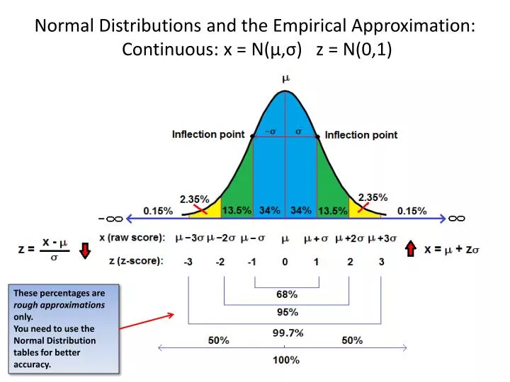
Normal Distributions and the Empirical Approximation: Continuous: x = N( μ , σ ) z = N(0,1). These percentages are rough approximations only. You need to use the Normal Distribution tables for better accuracy. §6.1. 6. What percentage of the area under the normal curve lies

E N D
Normal Distributions and the Empirical Approximation: Continuous: x = N(μ,σ) z = N(0,1) These percentages are rough approximations only. You need to use the Normal Distribution tables for better accuracy.
§6.1 • 6. What percentage of the area under the normal curve lies • To the right of μ?Greater than z = 0 so P = 50% • Between μ - 2σ and μ + 2σ? -2 < z < 2 so P = 95% • To the right of μ + 3σ? z > 3 so P = 0.15%
8. The incubation time for Rhode Island chicks is normally distributed with a mean of 21 days and standard deviation of approximately 1 day. • N(21,1): • If 1000 eggs are being incubated, how many chicks do we expect will hatch? • In 19 to 23 days? P(19 ≤ x ≤ 23) = P(-2 ≤ z ≤ 2) so P = 95%. Expect (.95)(1000) = 950 chicks. • (b) In 20 to 22 days? P(20 ≤ x ≤ 22) = P(-1 ≤ z ≤ 1) so P = 68%. Expect (.68)(1000) = 680 chicks. • (c) In 21 days or fewer? P(x ≤ 21) = P(z ≤ 0) so P = 50%. Expect (.50)(1000) = 500 chicks. • (d) In 18 to 24 days? -3 < z < 3 so P = 99.7%. Expect (.997)(1000) = 997 chicks.
10. A vending machine automatically pours soft drinks into cups. The amount of soft drink dispensed into a cup is normally distributed with mean of 7.6 ounces and standard deviation of 0.4 ounce. • N(7.6, 0.4): • Estimate the probability that the machine will overflow an 8-ounce cup. • P(x > 8.0) = P(z > 1) = 13.5 % + 2.35% + 0.15% = 16% • (b) Estimate the probability that it will not overflow an 8-ounce cup. • P(x ≤ 8.0) = P(z ≤ 1) = 100% - 16% = 84% • (c) The machine is loaded with 850 cups. How many of these do you expect will overflow when served? • (.16)(850) = 136 cups.
§6.2 • 8. Fawns between 1 and 5 months old in the Mesa Verde National Park have a body weight that is approximately normally distributed with mean μ = 27.2 kilograms and standard deviation σ = 4.3 kilograms. [ N(27.2, 4.3) ] Let x be the weight of a fawn. [ x is the raw score ] Convert each of the following x intervals to z intervals. • x < 30 (30 – 27.2) / 4.3 = 0.65 so z < 0.65 • (b) 19 < x (19 – 27.2) / 4.3 = -1.91 so -1.91 < z • (c) 32 < x < 35 (32 – 27.2) / 4.3 < z < (35 – 27.2) / 4.3 so 1.12 < z < 1.81 • Convert each of the following z intervals to x intervals. • (d) -2.17 < z 27.2 + (-2.17)(4.3) = 17.9 so 17.9 < x • (e) z < 1.28 27.2 + (1.28)(4.3) = 32.7 so x < 32.7 • (f) -1.99 < z < 1.44 27.2 +(-1.99)(4.3) < x < 27.2 +(1.44)(4.3) so 18.6 < x < 33.4 • (g) If a fawn weighs 14 kilograms, would you say it is unusually small? • z = (14 – 27.2) / 4.3 = -3.07. Yes, it’s unusually small.
The Standard Normal Probability Tables: z = N(0,1)z0 will always be some definite number: Left Table: P(z ≤ z0) for z0 ≤ 0 Right Table: P(z ≤ z0) for z0 0 Also use: P(z ≤ -3.50) = 0 P(z ≤ 3.50) = 1 P(z ≤ -1.23) = .1093
Standard Probability Calculations (pg 254) P(z ≤ z0) P(z < z0) P(z0 z) P(z0 > z) Read these directly from the Table P(z z0) P(z > z0) P(z0 ≤ z) P(z0 < z) = 1 - P(z ≤ z0) = P(z ≤ - z0) Or by symmetry: P(z0 ≤ z ≤ z1) P(z0 <z < z1) P(z1 z z0) P(z1 >z> z0) = P(z ≤z1) - P(z ≤z0)
§6.2 In Problems 29 – 48, let z be a random variable with a standard normal distribution. Find the indicated probability. 30. P(z ≥ 0) = 1 – P( z ≤ 0) = 1 - .5000 = .5000 32. P(z ≤ -2.15) = .0158 from the Table 34. P(z ≤ 3.20) = .9993 from the Table 40. P(-2.20 ≤ z ≤ 1.04) = P(z ≤ 1.04) – P(z ≤ -2.20) = .8508 - .0139 = .8369 42. P(-1.78 ≤ z ≤ -1.23) = P(z ≤ -1.23) – P(z ≤ -1.78) = .1093 - .0375 = .0718 44. P(0 ≤ z ≤ 0.54) = P(z ≤ 0.54) – P(z ≤ 0) = .7054 - .5000 = .2054
Example: A More Exact Empirical Approximation -3 -2 -1 0 1 2 3
Some Standard Symmetric Probabilities for z0 > 0 P(-z0 ≤ z ≤ z0) = P(|z| ≤ z0) = 1 - 2 P(z ≤ -z0) P(z z0or z ≤ - z0) = P(|z| z0) = 2 P(z ≤ -z0)
§6.3 In Problems 5 – 14 assume that x has a normal distribution with the specified mean and standard deviation. Find the indicated probabilities. The idea is simply to convert to z-scores, then look up the probabilities in the Table as in §6.2. 6. P(10 ≤ x ≤ 26); μ = 15; σ = 4 (10 – 15) / 4 ≤ z ≤ (26 – 15) / 4 so -1.25 ≤ z ≤ 2.75 P(10 ≤ x ≤ 26) = P(-1.25 ≤ z ≤ 2.75) = P(z ≤ 2.75) – P(z ≤ -1.25) = .9970 - .1056 = .8914 12. P(x ≥ 120); μ = 100; σ = 15 z ≥ (120 – 100) / 15 so z ≥ 1.33 P(x ≥ 120) = P(z ≥ 1.33) = 1 – P(z < 1.33) = 1 - .9082 = .0918
§6.3 26. Porphyrin is a pigment in blood protoplasm and other body fluids that is significant in body energy and storage. Let x be a random variable that represents the number of milligrams of porphyrin per deciliter of blood. In healthy adults, x is approximately normally distributed with mean μ = 38 and standard deviation σ = 12. [ N(38, 12) ] What is the probability that • x is less than 60? • Convert to z-scores: z < (60 – 38) / 12 = 1.83 • From the Table P(z ≤ 1.83) = .9664 • (b) x is greater than 16? • z > (16 – 38) / 12 = -1.83 • P(z > -1.83) = 1 – P(z ≤ -1.83) = 1 - .0336 = .9664 • (c) x is between 16 and 60? • P(-1.83 < z < 1.83) = P(z ≤ 1.83) – P(z ≤ -1.83) = .9664 - .0336 = .9328 • (d) x is more than 60? (This may indicate infection, anemia, or other type of illness) • P(z > 1.83) = 1 – P(z ≤ 1.83) = 1 - .9664 = 0.0336
The Normal Table is Also Available in Excel:§6.3 Prob 6 (Slide # 11): Make sure you put a “1” in the “cumulative” field No need to convert to z-scores: Excel does it for you from the μ and σ columns
§6.3 Prob 26 (Slide # 12) The difference between this answer and the previous one is that the Table in the book is rounded off to 4 places. Excel is much more accurate.
You can even compute things like P(z < 2) by setting x0 to a very small negative number like -1000 because P(z < 2) is the same thing as P(-∞ < z < 2) which is (basically) the same as P(-1000 < z < 2) … … and P(z > 2) by setting x1 to a very large positive number like 1000 because P(z > 2) is the same thing as P(2 < z < ∞) which is (basically) the same as P(2 < z < ∞)