Download
1 / 28
280 likes | 466 Views
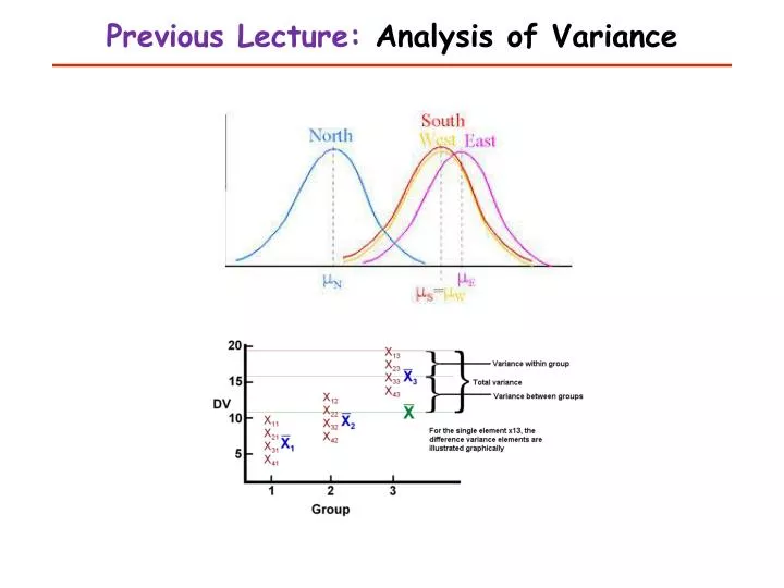
Previous Lecture: Analysis of Variance. This Lecture. Categorical Data Methods. Judy Zhong Ph.D. Outline. Categorical data Definition Contingency table Example Pearson’s 2 test for goodness of fit 2 test for two population proportions (Z test to compare two proportions)

E N D
This Lecture Categorical Data Methods Judy Zhong Ph.D.
Outline • Categorical data • Definition • Contingency table • Example • Pearson’s 2 test for goodness of fit • 2 test for two population proportions (Z test to compare two proportions) • 2 test of independence in a contingency table • Fisher’s exact test –small sample size
Categorical data • Definition: refers to observations that are only classified into categories so that the data set consists of frequency counts for the categories. • Example: • Blood type (O, A,B,AB) • A shipment of assorted nuts (walnuts, hazelnuts, and almonds) • Gender (male, female)
Example 1. Two population Proportions In a random sample, 120 Females, 12 were left handed; 180 Males, 24 were left handed
Example 2:Independent Samples classified in Several categories: • The meal plan selected by 200 students is shown below:
Contingency Tables Contingency Tables • Useful in situations involving multiple population proportions • Used to classify sample observations according to two or more characteristics • Also called a cross-classification table.
Pearson’s 2 test: for two population propotions(example 1) Sample results organized in a contingency table: sample size = n = 300: 120 Females, 12 were left handed 180 Males, 24 were left handed
2 Test for the Difference Between Two Proportions H0: p1 = p2 (Proportion of females who are left handed is equal to the proportion of males who are left handed) H1: p1 ≠ p2 (The two proportions are not the same – Hand preference is not independent of gender) • If H0 is true, then the proportion of left-handed females should be the same as the proportion of left-handed males • The two proportions above should be the same as the proportion of left-handed people overall
The Chi-Square Test Statistic The Chi-square test statistic is: • where: O = observed frequency in a particular cell E = expected frequency in a particular cell if H0 is true 2 for the 2 x 2 case has 1 degree of freedom (Assumed: each cell in the contingency table has expected frequency of at least 5)
Computing the Average Proportion The average proportion is: Here: 120 Females, 12 were left handed 180 Males, 24 were left handed i.e., the proportion of left handers overall is 0.12, that is, 12%
Finding Expected Frequencies • To obtain the expected frequency for left handed females, multiply the average proportion left handed (p) by the total number of females • To obtain the expected frequency for left handed males, multiply the average proportion left handed (p) by the total number of males If the two proportions are equal, then P(Left Handed | Female) = P(Left Handed | Male) = .12 i.e., we would expect (.12)(120) = 14.4 females to be left handed (.12)(180) = 21.6 males to be left handed
The Chi-Square Test Statistic The test statistic is:
Decision Rule Decision Rule: If 2 > 3.841, reject H0, otherwise, do not reject H0 Here, 2 = 0.7576 < 2U = 3.841, so we do not reject H0 and conclude that there is not sufficient evidence that the two proportions are different at = 0.05 0 2 Do not reject H0 Reject H0 2U=3.841
Test for Association for RxC Contingency Tables • Similar to the 2 test for equality of more than two proportions, but extends the concept to contingency tables with r rows and c columns H0: The two categorical variables are independent (i.e., there is no association between them) H1: The two categorical variables are dependent (i.e., there is association between them)
2 Test of Independence The Chi-square test statistic is: • where: O = observed frequency in a particular cell of the r x c table E = expected frequency in a particular cell if H0 is true 2 for the r x c case has (r-1)(c-1) degrees of freedom Assumed: 1. No cell has expected value < 1 2. No more than 1/5 of the cells have expected values < 5
Expected Cell Frequencies • Expected cell frequencies: Where: row total = sum of all frequencies in the row column total = sum of all frequencies in the column n = overall sample size
Decision Rule • The decision rule is If 2 > 2U, reject H0, otherwise, do not reject H0 Where 2U is from the chi-square distribution with (r – 1)(c – 1) degrees of freedom
Example • The meal plan selected by 200 students is shown below:
Example: Expected Cell Frequencies (continued) Observed: Expected cell frequencies if H0 is true: Example for one cell:
Example: The Test Statistic (continued) • The test statistic value is: 2U = 12.592 for = 0.05 from the chi-square distribution with (4 – 1)(3 – 1) = 6 degrees of freedom
Example: Decision and Interpretation (continued) Decision Rule: If 2 > 12.592, reject H0, otherwise, do not reject H0 Here, 2 = 0.709 < 2U = 12.592, so do not reject H0 Conclusion: there is not sufficient evidence that meal plan and class standing are related at = 0.05 0 2 Do not reject H0 Reject H0 2U=12.592
Fisher’s exact test • An alternative test comparing two proportions • compute exact probability of the observed frequencies in the contingency table • Under H0, it is assumed that there is no association between the row and column classifications and that the marginal totals remain fixed • Valid for tables with small expected cell values where the usual 2 test is not applicable. • At least one cell<5 • The exact test and the 2 test will give similar results where the use of the 2 test is appropriate.
Fisher’s exact test Example 10.17 in Rosner (p. 402)
Fisher’s exact test in R > table.CVD<-matrix(c(2,23,5,30), nrow=2,byrow=T) > table.CVD [,1] [,2] [1,] 2 23 [2,] 5 30 >fisher.test(table.CVD) Fisher's Exact Test for Count Data data: table.CVD p-value = 0.6882 alternative hypothesis: true odds ratio is not equal to 1 95 percent confidence interval: 0.04625243 3.58478157 sample estimates: odds ratio 0.527113
Summary • Categorical data • Contingency table • Pearson’s 2 test for goodness of fit • 2 test for two population proportions • 2 test of independence in a contingency table • Fisher’s exact test –small sample size