Understanding Sampling Distribution of Sample Proportions

1. Sampling Distribution of a Sample Proportion Lecture 27 Sections 8.1 – 8.2 Wed, Oct 25, 2006

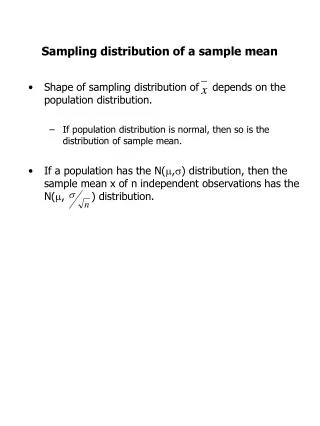
2. Preview of the Central Limit Theorem • We looked at the distribution of the sum of 1, 2, and 3 uniform random variables U(0, 1). • We saw that the shapes of their distributions was moving towards the shape of the normal distribution. • If we replace “sum” with “average,” we will obtain the same phenomenon, but on the scale from 0 to 1 each time.

3. Preview of the Central Limit Theorem 2 1 0 1

4. Preview of the Central Limit Theorem 2 1 0 1

5. Preview of the Central Limit Theorem 2 1 0 1

6. Preview of the Central Limit Theorem • Some observations: • Each distribution is centered at the same place, ½. • The distributions are being “drawn in” towards the center. • That means that their standard deviation is decreasing. • Can we quantify this?

7. Preview of the Central Limit Theorem • = ½ 2 = 1/12 2 1 0 1

8. Preview of the Central Limit Theorem • = ½ 2 = 1/24 2 1 0 1

9. Preview of the Central Limit Theorem • = ½ 2 = 1/36 2 1 0 1

10. Preview of the Central Limit Theorem • This tells us that a mean based on three observations is much more likely to be close to the population mean than is a mean based on only one or two observations.

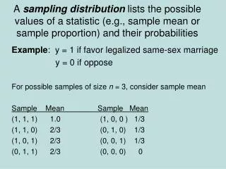
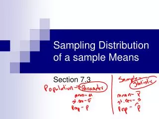
11. Parameters and Statistics • THE PURPOSE OF A STATISTIC IS TO ESTIMATE A POPULATION PARAMETER. • A sample mean is used to estimate the population mean. • A sample proportion is used to estimate the population proportion. • Sample statistics, by their very nature, are variable. • Population parameters are fixed.

12. Some Questions • We hope that the sample proportion is close to the population proportion. • How close can we expect it to be? • Would it be worth it to collect a larger sample? • If the sample were larger, would we expect the sample proportion to be closer to the population proportion? • How much closer?

13. The Sampling Distribution of a Statistic • Sampling Distribution of a Statistic – The distribution of values of the statistic over all possible samples of size n from that population.

14. The Sample Proportion • Let p be the population proportion. • Then p is a fixed value (for a given population). • Let p^ (“p-hat”) be the sample proportion. • Then p^ is a random variable; it takes on a new value every time a sample is collected. • The sampling distribution of p^ is the probability distribution of all the possible values of p^.

15. Example • Suppose that this class is 3/4 freshmen. • Suppose that we take a sample of 1 student. • Find the sampling distribution of p^.

16. F P(F) = 3/4 3/4 1/4 N P(N) = 1/4 Example

17. Example • Let X be the number of freshmen in the sample. • The probability distribution of X is

18. Example • Let p^ be the proportion of freshmen in the sample. (p^ = X/n.) • The sampling distribution of p^ is

19. Example • Now we take a sample of 2 student, sampling with replacement. • Find the sampling distribution of p^.

20. F P(FF) = 9/16 3/4 F 1/4 3/4 N P(FN) = 3/16 1/4 F P(NF) = 3/16 3/4 N 1/4 N P(NN) = 1/16 Example

21. Example • Let X be the number of freshmen in the sample. • The probability distribution of X is

22. Example • Let p^ be the proportion of freshmen in the sample. (p^ = X/n.) • The sampling distribution of p^ is

23. Samples of Size n = 3 • If we sample 3 people (with replacement) from a population that is 3/4 freshmen, then the proportion of freshmen in the sample has the following distribution.

24. Samples of Size n = 4 • If we sample 4 people (with replacement) from a population that is 3/4 freshmen, then the proportion of freshmen in the sample has the following distribution.

25. The Parameters of the Sampling Distributions • When n = 1, the sampling distribution is • The mean and standard deviation are •  = 3/4 = 0.75 • 2 = 3/16 = 0.1875

26. The Parameters of the Sampling Distributions • When n = 2, the sampling distribution is • The mean and standard deviation are •  = 3/4 = 0.75 • 2 = 3/32 = 0.09375

27. The Parameters of the Sampling Distributions • When n = 3, the sampling distribution is • The mean and standard deviation are •  = 3/4 = 0.75 • 2 = 3/48 = 0.0625

28. The Parameters of the Sampling Distributions • When n = 4, the sampling distribution is • The mean and standard deviation are •  = 3/4 = 0.75 • 2 = 3/64 = 0.046875

29. Sampling Distributions • Run the program Central Limit Theorem for Proportions.exe. • Use n = 30 and p = 0.75; generate 10000 samples.

30. 100 Samples of Size n = 30  = 0.75  = 0.079

31. Observations and Conclusions • Observation #1: The values of p^ are clustered around p. • Conclusion #1: p^ is probably close to p.

32. Larger Sample Size • Now we will select 10000 samples of size 30 instead of only 100 samples. • Run the program Central Limit Theorem for Proportions.exe. • Pay attention to the shape of the distribution.

33. 10,000 Samples of Size n = 30  = 0.75  = 0.0395

34. 10,000 Samples of Size n = 30

35. More Observations and Conclusions • Observation #2: The distribution of p^ appears to be approximately normal. • Conclusion #2: We can use the normal distribution to calculate just how close to p we can expect p^ to be.

36. Larger Sample Size • Now we will increase the sample size from 30 to 200 (and still generate 10000 such samples). • Run the program Central Limit Theorem for Proportions.exe. • Pay attention to the spread (standard deviation) of the distribution.

37. 10000 Samples of Size n = 200  = 0.75  = 0.0395

38. Observations and Conclusions • Observation #3: As the sample size increases, the clustering is tighter. • Conclusion #3-1: Larger samples give more reliable estimates. • Conclusion #3-2: For sample sizes that are large enough, we can make very good estimates of the value of p.

39. One More Conclusion • However, we must know the values of  and  for the distribution of p^. • That is, we have to quantify the sampling distribution of p^.

40. The Sampling Distribution of p^ • It turns out that the sampling distribution of p^ is approximately normal with the following parameters. • This is the Central Limit Theorem for Proportions, summarized on page 519.

41. The Sampling Distribution of p^ • The approximation to the normal distribution is excellent if

42. Why Surveys Work • Check out the latest poll results for the Virginia Senate race between George Allen and James Webb: http://www.realclearpolitics.com/latestpolls/ • If Webb really has 47% of the (decided) vote, what is the probability that a survey of 625 likely voters would show that he had only 43%?

43. Why Surveys Work • First, describe the sampling distribution of p^ if the sample size is n = 625 and p = 0.47. • Check: np = 293.75  5 and n(1 – p) = 331.25  5. • p^ is approximately normal.

44. Why Surveys Work • The z-score of 0.43 is • P(p^< 0.43) = P(Z< -2.004) = 0.0225 (not likely!) • Or use normalcdf(-E99, 0.43, 0.47, 0.01996).

45. Why Surveys Work • Perform the same calculation, but with a smaller sample size, say n = 50. • The probability turns out to be 0.2855, nearly a 30% chance! • By symmetry, there is also nearly a 30% chance that the sample proportion is greater than 51%. • Thus, there is nearly a 60% chance that the sample proportion is off by at least 4 percentage points.

46. The Margin of Error • For now, we can consider the margin of error to be 2 standard deviations. • In our example, with sample size n = 625, the margin of error is 2(0.01996) = 0.03992 = 3.992%. • With a sample size of n = 50, the margin of error is 2(0.07058) = 0.14116 = 14.116%.