Download
1 / 39
420 likes | 484 Views
Job Shop Scheduling. Job shop environment : m machines, n jobs objective function Each job follows a predetermined route Routes are not necessarily the same for each job Machine can be visited once or more than once (recirculation). Job Shop Problem Network Formulation.

E N D
Job shop environment: • m machines, n jobs • objective function • Each job follows a predetermined route • Routes are not necessarily the same for each job • Machine can be visited once or more than once (recirculation)
Job Shop ProblemNetwork Formulation • Let us consider the example with 4 m/c & 3 jobs • The route of the jobs as well as their processing times are given below Jobm/c sequenceProcessing time 1 1- 2 -3 P11=10 P21=8 P31=4 2 2-1-4-3 P22=8 P12=3 P42=5 P32=6 3 1-2-4 P13=4 P23=7 P43=3 where Pij job J processed on m/c i
Construction of the Network 1,1 2,1 3,1 0 0 0 S 2,2 1,2 4,2 3,2 T 1,3 2,3 4,3
Problem :Jm | | Cmax Node (i, j) represents the operation of jth job on ith machine • Pij processing time of job j on machine i • G = (N, AB) • A: Solid (Conjunctive) arcs represent the precedence relationships between operation of a single job. • Operation (i, j) precedes (k, j)
B: Broken (Disjunctive) arcs represent the precedence relationships between operation of a single machine. • Disjunctive arcs B represent conflicts on machines. • Two operations (i, j) and (i, l) are connected by two arcs going in opposite direction. • Two dummy nodes S and T representing source and sink. • Arcs from S to all first operations of jobs. • Arcs from all last operations of jobs to T • A feasible schedule corresponds to a selection of at most one (disjunctive) broken arcs from each such pair such that the resulting directed graph is acyclic
How to construct a feasible schedule? Select D - a subset of disjunctive arcs (one from each pair) suchthat the resulting directed graph G(D) has no cycles. Graph G(D) contains conjunctive arcs + D. D represents a feasible schedule. A cycle in the graph corresponds to a schedule that is infeasible.
10 8 1,1 2,1 3,1 4 0 0 8 3 5 6 S 2,2 1,2 4,2 3,2 T 3 0 4 7 1,3 2,3 4,3 • The makespan of a feasible schedule is determined by the longest path in G(D) from S to T. • Minimise makespan: find a selection of disjunctive arcs that minimises the length of the longest path (the critical path).
Selection • A subset is called a selection if it contains from each pair of disjunctive arcs exactly one. • A selection D is feasible if the resulting directed graph G (D) = (N, A D) i.e. graph with conjunctive and selected disjunctive arcs is acyclic.
Remarks • A feasible selection leads to a sequence in which operations have to be processed on machines. • Each feasible selection leads to a feasible schedule.
Ex. Machines – M1, M2, M3 Jobs J1 where (3, 1) (2, 1) (1, 1) J2 where (1, 2) (3, 2) J3 where (2, 3) (1, 3) (3, 3) Duration P31 = 4 P21 = 2 P11 = 1 P12 = 3 P32 = 3 P23 = 2 P13 = 4 P33 = 1
3,1 2,1 1,1 u 1,2 3,2 v 2,3 1,3 3,3 Feasible Selection Represents conjunctive arcs Selection
M1 J3 J1 J2 Corresponding Schedule M2 J1 J3 M3 J1 J2 J3 5 10 15 20 Make Span Cmax = 20
3,1 2,1 1,1 u 1,2 3,2 v 2,3 1,3 3,3 Selection for given schedule Selection
M1 J2 J1 J3 M2 J3 J1 M3 J1 J2 J3 5 10 12 Make Span Cmax =12
Disjunctive Programming Formulation Minimizing Cmax Subject to where yij denotes starting time of operation (i, j) } for all Cmax for all for all (i, l) & (i, j) i = 1, 2, …..,m for all
Some ordering must exists among operation of different job that are processed on same machine. • Solution procedures for Jm / Cmaxare based either on enumerative or heuristic. • No standard solution procedure available that will work satisfactory. • Two popular heuristic algorithms: (i) schedule generation algorithm. (ii) shifting bottleneck heuristic algorithm;
Algorithm for Non Delay Schedule Generation - A partial schedule containing t scheduled operations - The set of schedulable operations at stage t corresponding to a given - The earliest time at which operation could be started - The earliest time at which operation could be completed
is determine by the completion time of the direct predecessor of operation J and latest completion time on the machine required by operation J • The larger of these quantities is • The potential finish time where is processing time of operation J Here (i, j, k) represents job i operation J on machine k
Algorithm Step 1 – Let t = 0 and includes all operations with no predecessor. Step 2 – Determine and the machine on which could be realized Step 3 – For each operation that requires machine and for which create a new partial schedule in which operation J is added to and started at time
Step 4 – For each new partial schedule created in step 3, update the data set as follows (a) Remove operation J from (b) Form by adding the direct successor of operation J to (c) Increment t by 1 Step 5 – Return to step 2 for each created in step 3 and continue in this fashion until all non delay schedules have been generated. • The quality of the solution obtained by the heuristic mainly depends on the effectiveness of priority rules which are used in them.
A Sample Set of Priority Rules • SPT – Select the job with min. processing time • FCFS – Select the operation that entered earliest • MWKR – (Most work remaining) – Select the operation associated with the job having the most work remaining to be processed • MOPNR – (Most operation remaining) – Select the operation that has the largest number of successor operation • Random – Select the operation at random
Ex. Find the schedule using non delay schedule generation heuristic with following primary rules First level priority rule – MWKR (Most work remaining) Second level priority rule – SPT Third level priority rule – Random order
Operation Operation 1 2 3 1 2 3 Job Job 1 2 3 4 1 2 3 4 • 3 4 • 4 4 1 • 2 3 • 3 3 1 • 1 2 3 • 3 2 1 • 2 3 1 • 1 3 2 Processing timeRouting
Job Operation At t = 0 for all M/c Earliest time at which operation could be started *Therefore, priority rule must be involved to select among all four operation [MWKR]
R1= 9R2= 9R3= 7R4= 7 • MWKR = 9 is not unique. • This is occurring for job 1 and job 2 • Now, a tie breaking rules is needed • SPT is used as tie breaking rule • Now t111 < t213
M/c1 (1, 1, 1) M/c2 M/c3 2 4 6 • This means PS1 consists of operation {(1, 1, 1)} started at time 0 PS1 = {(1, 1, 1)} f1 = 2, f2 = 0, f3 = 0
At this stage for two operations in S1. Thus priority rule must be involved to choose between (2, 1, 3) and (3, 1, 2)
M/c1 (1, 1, 1) M/c2 M/c3 (2, 1, 3) 2 4 6 By applying MWKR, we get R2 = 9 R3 = 7 since R2 > R3 (2, 1, 3) is added to PS1 to form PS2 = {(1, 1, 1), (2, 1, 3)} f1 = 2, f2 = 0, f3 = 4
Now Operation 1 of job 2 is to be completed in M/c 3
M/c1 (1, 1, 1) M/c2 (3, 1, 2) M/c3 (2, 1, 3) 2 4 6 *The minimum is for & it is unique. Add this to partial schedule PS3 PS3 = {(1, 1, 1), (2, 1, 3), (3, 1, 2)} f1 = 2, f2 = 2, f3 = 4
At this stage for two operation • Thus priority rule must e involved to choose between (1, 2, 2) and (4, 1, 1) R1 = 7 R4 = 7 • MWKR is not unique. • Now SPT is used as tie breaker & t122 = t411 • After it is resolved randomly in favor of (4, 1, 1) PS4 = {(1, 1, 1), (2, 1, 3), (3, 1, 2), (4, 1, 1)} f1 = 5, f2 = 2, f3 = 4
S4 = {(1, 2, 2), (2, 2, 2), (3, 2, 3), (4, 2, 3)} Operation 1 of job 4 in M/c 1 takes 5 minutes
Now (1, 2, 2) is added to PSt • Thus PS5 = {(1, 1, 1), (2, 1, 3), (3, 1, 2), (4, 1, 1), (1, 2, 2)} f1 = 5, f2 = 5, f3 = 4 Now S5 = {(1, 3, 3), (2, 2, 2), (3, 2, 3), (4, 2, 3)}
This minimum corresponds to (3, 2, 3) only partial schedule PS6 = {(1, 1, 1), (2, 1, 3), (3, 1, 2), (4, 1, 1), (1, 2, 2), (3, 2, 3)} • In this way we have to proceed to stage to complete the entire schedule The final schedule is given as P12 = {(1, 1, 1), (2, 1, 3), (3, 1, 2), (4, 1, 1), (1, 2, 2), (3, 2, 3) (2, 2, 2), (2, 3, 1), (4, 2, 3), (3, 3, 1), (1, 3, 3), (4, 3, 2)}
M/c1 (1, 1, 1) (4, 1, 1) (2, 3, 1) (3, 3, 1) 2 5 9 10 13 M/c2 (3, 1, 2) (1, 2, 2) (2, 2, 2) (4, 3, 2) 2 M/c3 (2, 1, 3) (3, 2, 3) (4, 2, 3) (1, 3, 3)
Further Reading 1. Scheduling, Theory, Algorithms, and Systems, Michael Pinedo, Prentice Hall, 1995, or new: Second Addition, 2002 Chapter 6 or 2. Operations Scheduling with Applications in Manufacturing and Services, Michael Pinedo and Xiuli Chao, McGraw Hill, 2000Chapter 5