Download
1 / 32
320 likes | 467 Views
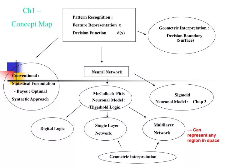
Ch1 – Concept Map. Pattern Recognition : Feature Representation x Decision Function d(x). Geometric Interpretation : Decision Boundary. (Surface). Neural Network. Conventional : Statistical Formulation - Bayes : Optimal Syntactic Approach.

E N D
Ch1 – Concept Map Pattern Recognition : Feature Representation x Decision Function d(x) Geometric Interpretation : Decision Boundary (Surface) Neural Network Conventional : Statistical Formulation - Bayes : Optimal Syntactic Approach McCulloch–Pitts NeuronalModel : Threshold Logic Sigmoid Neuronal Model : Chap 3 Multilayer Network Single Layer Network Digital Logic → Can represent any region in space Geometric interpretation
Class Recognition : Image -> Apple Two Objectives Attribute Recognition – Image -> Color, Shape, Taste, etc. Chapter 1. Pattern Recognition and Neural Networks 1. Pattern Recognition Ex. Color (attribute) of apple is red. (1) Approaches Statistical a. Template Matching ω P ( x ) b. Statistical 2 ω P ( x ) 1 c. Syntactic d. Neural Network x Class 1 Class 2 Bayes Optimal Decision Boundary Ex. x = temperature, ω1: healthy, ω2 : sick. x = (height, weight), ω1: female, ω2:male.
(2) Procedure - Train and Generalize Raw x x d ( ) Preprocessing Feature Extraction Discriminant Decision making Class Data Eliminate bad data (outliers) Filter out noise For data reduction, better separation Training Data = Labelled Input/Output Data = { x | d(x) is known }
(3) Decision ( Discriminant) Function a. 2-Class Weather Forecast Problem n = 2, M = 2 x 2 w 2 = = decision boundary x w d ( ) 0 1 = ( n-1) dim . = line, plane, hyperplane. x1 = temp, x2 = pressure x 1 unnormalized normalized w1 w2 w3
T w x 0 > w x D T 0 < < T 0 w x D 0 < T w x 0 0 In general, x w 0 D = T w x D 0 is a unit normal to the Hyperplane. T x = w 0 0
+ - - + - + b. Case of M = 3 , n = 2– requires 3 discriminants Pairwise Separable - Discriminants Req.
Max Max Max Linear classifier Machine
d 3 w w w w 1 3 1 3 IR d2 = d 0 w 23 2 = d w 0 d 1 2 1
2. PR – Neural Network Representation (1) Models of a Neuron A. McCulloch-Pitts Neuron – threshold logic with fixed weights 1 x x w 1 -q = bias 1 1 x j w 2 ) S x ( u` = j y 2 u 2 M q M x w p p Adaptive Linear Combiner Nonlinear Activation Function x p (Adaline)
- q q B. Generalized Model Half Plane Detector w bias x 1 1 w 2 + x 2 -w bias x 1 1 ? -w 2 x 2 j j j Ramp Logistic One-Sided Hard Limiter, Threshold Logic Binary Piecewise Linear j j j Ramp Signum, Threshold Logic tanh Two-Sided Bipolar
(2) Boolean Function Representation Examples x , x = binary (0, 1) 2 1 x x 1 1 OR AND 1.5 0.5 x x 2 2 x x -1 -1 1 1 NAND -1.5 NOR -0.5` -1 -1 x x 2 2 1 Excitatory 1 -1 x INVERTER -0.5 0.5 MEMORY 1 -1 Inhibitory Cf. x , x may be bipolar ( -1, 1) → Different Bias will be needed above. 1 2
x 1 x 2 (3) Geometrical Interpretation A.Single Layer with Single Output = Fire within a Half Plane for a 2-Class Case B. Single Layer Multiple Outputs – for a Multi-Class Case w w w 1 2 3 1 0 0 0 1 0 0 0 1
C. Multilayer with Single Output - XOR Nonlinearly Separable Linearly Nonseparable → Bipolar Inputs, Other weights needed for Binary Representation. x 3 1 OFF ON 1 x 0 2 -5 x x 1 2
AND - 1 x -1.5 1 1 XOR 1.5 - 1 1 1 x 0.5 2 1 ) j ( x x + - 2 1 x x x =0.5 x =0.5 + - - 2 2 1 1 a. Successive Transforms - 1 NAND OR x 0.5 1 XOR 1 0.5 1 x 0.5 2 - 1 OR j x ( ) x x x - - x 2 1 1 2 2 x x x - + 2 1 1
x 1 AND OR b. XOR = OR ─ (1,1) AND 1 1 -2 1.5 0.5 1 1 x 2 c. Parity 1 x x 0.5 0.5 1 1 1 1-bit parity 0.5 1 1 1 x -1 x 1.5 1.5 = XOR 2 2 1 -1 n-bit parity 0.5 n+1 (-1) x n-0.5 n
D. Multilayer with Single Output – Analog Inputs (1/2) 1 1 1 1 OR OR 2 2 3 2 2 3 1 1 AND 2 2 3 3
E. Multilayer Single Output – Analog Inputs – (2/2) 1 2 5 AND 1 2 4 3 5 OR 6 4 6 3 1 1 2 AND 2 3 3 OR 4 4 AND 5 5 6 6
XOR Interwined General A B 1-layer: Half planes A B B A A B 2-layer: Convex A B B A 3-layer: Arbitrary A B A B B A MLP Decision Boundaries
2 2 ② 2 2 1 ② 1 1 ① ① 0 1 1 0 1 0 1 1 1 Exercise : Transform of NN from ① to ② : See how the weights are changed. 2 1 ① ② 0 1 2 3 1
Questions from Students -05 • How to learn the weights ? • Any analytic and systematic methodology to find the weights ? • Why do we use polygons to represent the active regions [1 output] ? • Why should di(x) be the maximum for the Class i ?